Solving Problems

Learning Objectives

Following this assignment students should be able to:

Combine multiple computing concepts to solve bigger problems

Identify and debug errors in code

Use online tools to help understand bugs in your code and resolve them

Reading

Topics

Problem decomposition
Basic debugging
Asking for help
Debugging with generative AI

Readings

Nick Cox’s Speaking Stata: How to debug, part I

Lecture Notes

Exercises

Understand the Problem (10 pts)

For the first three exercises this week we will use a common goal problem:
Goal problem: Starting from plot_dataset.dta (one row per plot), create a household dataset with:
- one observation per hh_id_merge
- mean plot yield (kg/ha) per household
- total nitrogen (kg) per household
- total labor (days) per household
- the number of plots managed by the household in that season
- an indicator for whether the household had any irrigated plot that season
Your job in this exercise is not to solve this problem. Your job is to understand and define it clearly. Complete the following steps, using comments to record your answers.

1. Restate the problem in your own words. Under the heading for this exercise, write a short paragraph (1–3 sentences) as comments that restates the goal problem in your own words. Your restatement should mention:
- What the starting data look like (plot-level)
- What the final data should look like (household–level)
- The key variables you need to create
2. Identify the inputs. Next, think about what information you need to solve the problem.
- Load the data just to inspect its structure
- In comments, list the inputs you think you need
3. Identify the desired outputs. In comments, explain:
- what each row of the final dataset represents,
- what variables the final dataset should contain,
- whether you expect to save this final dataset, and if so:
  - file name, and
  - location (e.g., in $export).
4. Ask clarification questions. Finally, imagine you are about to start writing code but your collaborator is online. What questions would you ask before you start? Add at least three clarifying questions as comments.
Break the Problem Down (10 pts)

Using the same goal problem, your job in this exercise is to build a structured plan (essentially an outline of the steps you will take to solve the problem) using house-style headings, bookmarks, and comments. You do not need to write any new Stata commands beyond headings and comments. Rather, you are building a plan, not writing full code. Do not implement the commands yet. You will start coding in Exercise 3.

1. Create high-level headings. Using the house style, create a set of major (**#) and minor (**##) sections that could solve the goal problem. The headings should: - Cover the full workflow from raw data to final dataset, and - Follow house style (**# for headings, **## for subheadings)

2. Add “mini-steps” under one heading. Pick one of your big sections (for example, “collapse to household level”) and break it down into smaller steps using comments.
One Piece at a Time (10 pts)

In this exercise, you will implement only the early steps of the plan you made in exercise 2 and one small piece at a time instead of trying to solve everything at once. Again, using the goal problem defined in exercise 1, complete the steps below, running and checking each block as you write it.

1. Load and inspect the data. Use use, describe, and sum. After running this block, add a short comment describing what you learned.

2. Create per-plot variables. Create at least one per-plot variable that you expect to use later. A natural example is yield per hectare but you can choose the variable you want to create, as long as it fits into the goal problem and plan you outlined in exercise 2.
Debugging (20 pts)

In this exercise you will practice systematic debugging using a deliberately broken .do file that works with plot_dataset.dta. Your goals are to:
- Make the bug reproducible from a clean session.
- Fix one bug at a time, always reading the error message.
- Use Stata’s tools (describe, sum, list, help r(###), etc.) to understand what’s going on.
- End with a clean, working script and a short reflection.
At the top of this exercise make sure you can reproduce errors from a clean session. To do this type
```
    clear              all
    do                 "$code/projectdo.do"
```
Run this script. Then copy the following broken code block directly after the line where you run the projectdo file.
```
******************************************************************
**# 1 - plot-level yield summaries
******************************************************************

* load data
    use             "$root/plot_dataset", clear

* create yield per hectare
    gen             yield_ha = harvestkg / plot_area_GPS

* summarize average yield for irrigated plots only, by main crop
    bys             main_crop: sum yield_ha if irrigated = 1, details

******************************************************************
**# 2 - save irrigated-only data by agro-ecological zone (aez)
******************************************************************

* get list of aezs
    levelsof        aez, local(agro_ecological_zone)

* loop over aezs and save a file for each
    foreach s of local agro_ecological_zone {

    * keep only irrigated plots for this aez
        keep        if agro_ecological_zone == s & irrigated == 1

    * save aez-specific file
        save        "$export/plot_yield_irr_s.dta"

    * reload data for next loop iteration
        use         "$root/plot_dataset.dta", clear
    }
```
There are multiple bugs in this code (file names, variable names, = vs ==, loop logic, options, and more). Do not fix anything yet. Run your assignment_7.do file from the top and let Stata stop at the first error.

For each bug you encounter:
- Run your .do file from the top until Stata stops with an error.
- Copy the error message and code in a comment below the offending line using the pattern (tabbed in twice):
```
*** ERROR HERE: r(111) type mismatch; harvestkg does not exist
```
Comment out the broken code and immediately below that *** comment decribing the error fix the bug. Then run the file from the top again to see the next error. Repeat this process until the entire script runs without errors. You should end up with a series of *** ERROR HERE: comments documenting each bug you found followed by your debugged code.

As you debug, remember to use Stata’s tools at appropriate points (do not use online help or an LLM).
- describe
- sum or sum, detail
- list or browse
- tab
- help r(###) for the error codes you encounter
- display of a macro (e.g., display "`s'") or returned result (e.g., display r(mean))
Each time you use one of these tools, add a short *** comment summarizing what you learned.

When you have completed this exercise you should have all the broken code commented out, followed by your comments regarding what the problem/bug was, and then a cleaned, working version of the buggy code block.
Stata Help (10 pts)

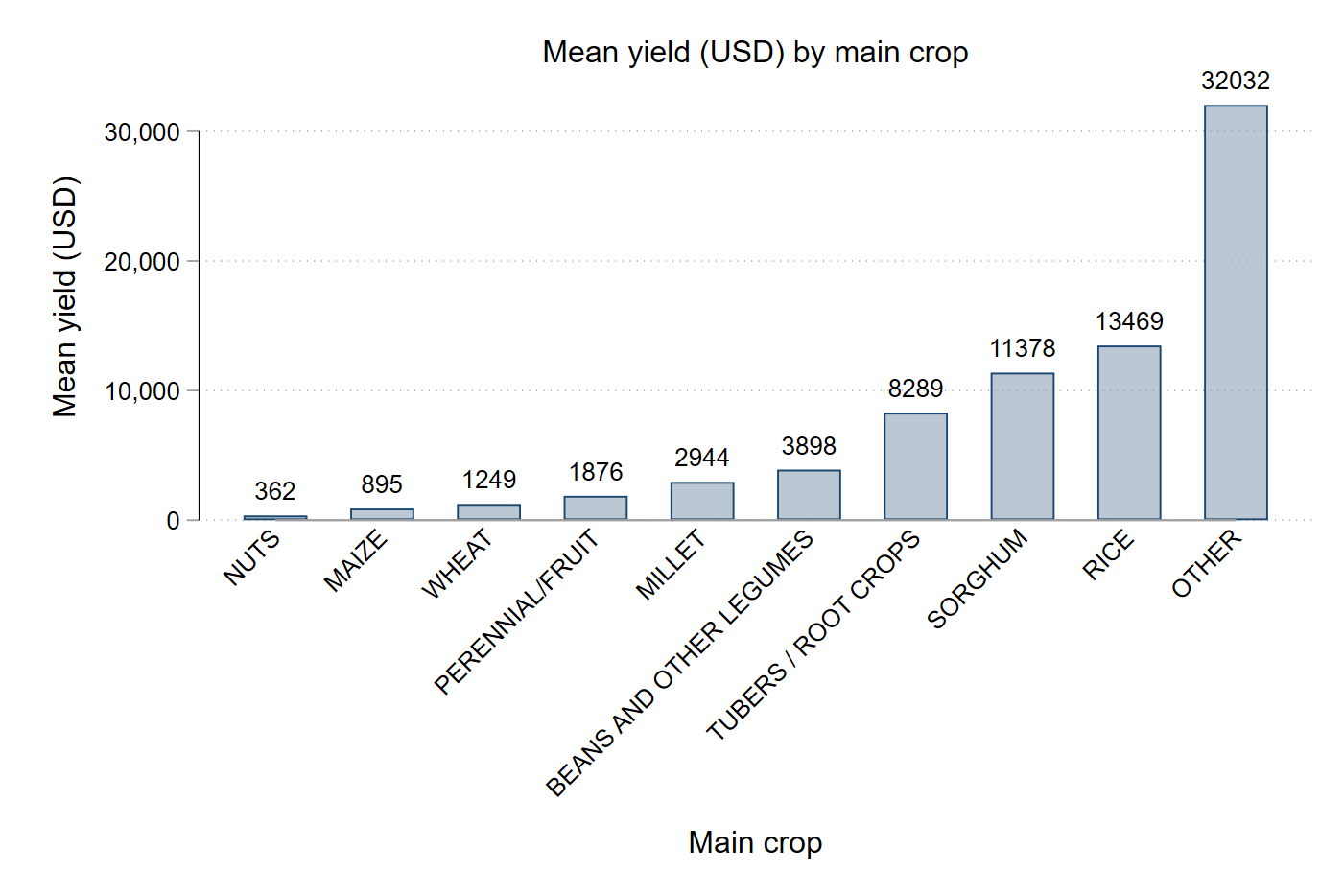
In this exercise you will practice using Stata’s built-in help and documentation to solve a concrete coding problem. Using plot_dataset.dta you need to create a graph of mean yield per hectare by main crop, with bars sorted from lowest to highest mean yield. You are expected to use help or search inside Stata to figure out the exact syntax and options. You are not to use online sources or LLMs.

1. Load the plot_dataset.dta and create and label a variable called yield_USD which is harvest_value_USD divided by plot_area_GPS. Summarize the variable and below that command add a *** comment that records the mean, standard deviation, min and max values.

2. Use help graph bar (or another relevant help file) to create a bar graph that displays mean yield by main_crop sorted from lowest to highest mean yield. As you code answer questions like:
- How do I compute mean of a variable in a graph bar command?
- How do I put different groups on the x-axis?
- How can I sort the bars by the mean value?
- How can I add axis titles and an overall title?
Record key options you decide to use in comments as well as summaries of what you learned from help. The exact graphing options are up to you, as long as they work and are informed by the help file.
Online Help (10 pts)

In this exercise you will practice using online resources (Statalist, Stack Overflow, etc.) to solve a coding problem and adapt example code safely. For exercise 1-3 you developed and partially implemented a plan to turn the plot-level data set into a household-level data set. In laying out that plan you most likely proposed using the collapse function to aggregate each row (plot) into a new data set where each row represented a household.

You need to use the Statalist and/or Stack Overflow to find a way to create a data set that allows you to analyze household-level information without losing the plot-level information (as would happen with collapse). Essentially, the plot_dataset.dta has a hierarchical structure: plots (level 1, L1) are clustered in households (level 2, L2). We want to analyze the L2 only values (by aggregation of the L1 values) by keeping just one value for each L2 unit without using collapse so that we de facto have two datasets in one.

1. Go to Statalist and search within the forum for something like:
- egen tag by group mean
- egen tag() keep one per group
- egen mean by() tag()
Find a post where someone demonstrates tagging one row per group (for example, Nick Cox’s example using egen tag = tag(groupvar)). Then adapt that code so that you keep the plot-level data set AND have household-level data.
- For each household, calculate mean yield_USD, total_labor_days, and nitrogen_kg Call these new variables mean_yield, tot_labor, and tot_fert.
- Then create a variable that tags a single observations per household and call it tag_hh.
- Label all four variables that you created.
In addition to your code, add to your .do file a short comment block documenting what you used similar to:
```
* online search:
* - search terms:
* - website/post used: statalist (general stata discussion)
* - key idea learned: compute group stats with egen, then egen tag = tag(groupvar)
*   and keep only tag==1 to get one row per group
```
How many observations are tagged with a 1?

2. To verify that you adapted the code correctly, run a regression with the household mean yield on the left-hand side and household total labor days and nitrogen fertilizer on the right-hand side. What are the coefficients on tot_labor and tot_fert?

LLM Help (20 pts)

In this exercise you will practice using a large language model (LLM) (e.g., ChatGPT, Copilot) to help debug or understand a small piece of Stata code. The point is not to have the LLM do the assignment for you. Instead, you will:

Write a short piece of Stata code that actually produces an error or surprising result when run with plot_dataset.dta
Ask an LLM for help understanding and fixing that specific issue
Implement the fix and verify it works

Copy and paste the following code into your .do file.

* load data
	use             "$data/plot_dataset.dta", clear

* keep maize only (main_crop is string)
	keep            if main_crop == MAIZE

* base restrictions
	keep            if plot_area_GPS > 0
	keep            if harvest_kg < .
	drop            if harvest_kg <= 0

* get list of countries
	levelsof        country, local(countries)

* make sure grc1leg2 is available
	cap which       grc1leg2
	if              _rc != 0 {
		net         install grc1leg2, ///
					from("https://fmwww.bc.edu/RePEc/bocode/g") ///
					replace
	}

* locals to store graph names (separate lists)
	local           glist_rf ""
	local           glist_ir ""

	local           leg_rf   ""
	local           leg_ir   ""

* loop over countries and irrigation status (0/1)
foreach `c' of local countries {

	foreach irr in 0 1 {

		preserve

		* restrict to this country + irrigation group
			keep if 		country == `c' & ///
								irrigated = `irr'

		* skip empty groups
			count
			if              r(N) = 0 {
				restore
				continue
			}

		* winsorize harvest (p1-p90 within group)
			_pctile         harvest_kg p(1 90)
			local           p1  = r(r1)
			local           p90 = r(r2)

			gen             harvest_kg_g = harvest_kg
			replace         harvest_kg_g = `p1'  ///
								if harvest_kg_g < p1
			replace         harvest_kg_g = `p90' ///
								if harvest_kg_g > `p90'
			lab var         harvest_kg_g "harvest winsorized (p1-p90)"

		* labels + short graph name
			local           irr_lbl "rainfed"
			if              `irr' == 1 local irr_lbl irrigated

			local           gname "g_ma_`c'_`irr"

		* color schemes by irrigation status
			local           mcol ""
			local           lcol1 ""
			local           lcol2 ""

			if              `irr' == 0 {
				local       mcol  "navy%25"
				local       lcol1 "midblue"
				local       lcol2 "eltblue"
			}
			if              `irr' == 1 {
				local       mcol  "dkgreen%25"
				local       lcol1 "forest_green"
				local       lcol2 "lime"
			}

		* create graph (do not export individual files)
			twoway         (scatter harvest_kg_g plot_area_GPS ///
								msize(tiny) mcolor(`mcol') ) ///
							(lfit harvest_kg_g plot_area_GPS, ///
								lcolor(`lcol1') lw(medthick) ) ///
							(lowess harvest_kg_g plot_area_GPS, ///
								lcolor(`lcol2') lw(medthick) ///
								bwidth(.8)), ///
							title("Harvest vs. plot area: `c' (`irr_lbl')", ///
								size(small))
							xtitle("plot area (gps)", ///
								size(small)) ///
							ytitle("harvest (kg)", ///
								size(small) margin(small)) ///
							xlabel(, labsize(small)) ///
							ylabel(, labsize(small)) ///
							legend(order(1 "plots" 2 "linear fit" ///
								3 "lowess") ///
								rows(1) position(3) ring(0) ///
								region(lstyle(none)) ) ///
							name(`gname' replace)

		* add graph to the appropriate combine list
			if              `irr' == 0 {
				if          "`glist_rf'" == "" local leg_rf "`gname'"
				local       glist_rf `"`glist_rf' `gname'"'
			}
			if              `irr' == 1 {
				if          "`glist_ir'" == "" local leg_ir "`gname'"
				local       glist_ir `"`glist_ir' `gname'"'
			}

		restore
	}
}

* combine rainfed graphs
	grc1leg2        `glist_rf', ///
						col(2) row(`rows_rf') ///
						xcommon ycommon ///
						imargin(tiny) ///
						graphregion(margin(zero)) ///
						legendfrom(`leg_rf')

	graph           export "$answ/07-llm-help-2.pdf" replace

* combine irrigated graphs
	grc1leg2        `glist_ir', ///
						col(2) row(`rows_ir') ///
						xcommon ycommon ///
						imargin(tiny) ///
						graphregion(margin(zero)) ///
						legendfrom(`leg_ir')

	graph           export "$answ/07-llm-help-3.pdf" replace

1. Run this block and confirm that it fails or produces unexpected output. What is the first error message do you get?

2. Outside of Stata, open an LLM (e.g., ChatGPT, Copilot) and:

Explain briefly what you are trying to do.
Paste your short code snippet.
Include the exact error message or describe the unexpected result.

In your .do file, summarize what you asked and the LLM’s response. Do not paste the full conversation into your .do file—just your own summary.

**## 7.2 - what i asked the llm

* in 2–4 sentences, summarize:
* - what task you described
* - what code you showed
* - what error or odd behavior you reported
* - what the llm thought the problem was
* - what fix or explanation it suggested

3. Write a corrected version of your code, using the LLM’s suggestion (possibly with your own modifications)

Check That Your Code Runs (10 pts)

Sometimes you think you’re code runs, but it only actually works because of something else you did previously. To make sure it actually runs you should save your work and then run it in a clean environment.

Follow these steps in to make sure your code really runs:
1. Restart Stata by closing the instance of Stata that you have open.
2. When you reopen Stata, type in the command line clear all. Or, better yet, put clear all at the top of your .do file, after the preamble but before any commands.
3. Rerun your entire homework assignment by clicking the Execute button to make sure it runs from start to finish and produces the expected results.
4. Make sure that you saved your code with the name of the assignment number (i.e., assignment_01). You should see the file in your git repo on your machine.
5. Make sure that your code will run on other computers (relevant for all assignments after the first assignment)
  - No cd. Use a project.do file instead to set directories
  - Use only relative paths in files other than the project.do file
  - Use / not \ for paths
Challenge 7 (Challenge - 20 pts)

For this challenge you are going to take the plot_dataset and create a household-level analysis dataset (one row per hh_id_merge). This is essentially the “goal problem” from this week, but here you will carry it to completion. In building the household-level data set, you are not allowed to use collapse.

1. Plan first (problem decomposition in your .do file). Before writing real code, create a section where you plan the solution using headings and comments only.
- Restate the problem in your own words
- Identify inputs/outputs
- Break into steps (load → construct variables → aggregate/tag → check uniqueness → analysis → graphs → save)
2. Build the household dataset.
- Start by dropping all observations that are not maize
- Instead of using collapse, use egen to compute household-level statistics for the following: - hh_id_merge - mean_yield = mean of plot-level yield_USD - tot_labor = sum of total_labor_days - tot_fert = sum of nitrogen_kg - n_plots = count of plots per household - any_irrig = 1 if household has any plot with irrigated==1, else 0
- Label each variable
- Tag one observation per household using the tag function
- Use keep if to keep one row per household. How many observations are now in the data set?
3. Check that following and include *** comments recording the mean of each variable and the number of irrigated plots:
- Confirm the dataset is one row per household: isid hh_id_merge
- Summarize mean_yield, tot_labor, tot_fert, n_plots
- Tabulate any_irrig
4. Run the regressions reg mean_yield tot_labor tot_fert any_irrig. Add *** comments that report:
- The sign of each coefficient
- One sentence interpreting the coefficient on any_irrig
5. Create two graphs.
- A twoway scatter plot of household mean yield (y-axis) vs total fertilizer (x-axis). Overlay a linear fit (lfit) to the data and provide informative axis titles and a legend.
- Create a bar chart of mean household yield by irrigation status (over). Bars are for any_irrig==0 and any_irrig==1 and the y-axis should be the mean of mean_yield.

Assignment submission checklist

Assignment