Research Design

Learning Objectives

Following this assignment students should be able to:

Describe how to design research in order to answer a causal question

Identify causal effects versus correlational relationships

Describe an identification strategy using causal diagrams (DAGs)

Reading

Topics

Research design
Identification
Causal diagrams

Readings

Reading (chapter 1): The Effect
Reading (chapter 5): The Effect
Reading (chapter 6): The Effect

Lecture Notes

Exercises

Simulating a Confounded DGP (20 pts)

In this exercise we are going to practice simulating a confounded DGP and diagnosing bias.
- Set the random seed to 24601 and simulate 30,000 observations.
- Generate an unobserved confounder called ability that is distributed Normal(0, 1)
- Generate a variable called p_train using a probability rule (invlogit) that increases with ability: invlogit(-0.2 + 1.0*ability)
- Then assign training as a Bernoulli draw train = (runiform() < p_train)
- Create a variable eps ~ rnormal(0, 3) so there is meaningful noise
- Generate wages so that the true causal effect of training be +2 and ability raises wages by +4 while wages without training (train = 0) or ability (ability = 0) is 10
- Add noise to the wage equation so that wage_lat = 10 + 2*train + 4*ability + eps
- Enforce wage >= 0 by truncating at 0 using max(wage_lat, 0)
- Add variable labels to all variables and value labels for train (0 = no, 1 = yes)
1. What is the naive difference in means by training status and is it larger or smaller than the true causal effect?
- Compute the naive difference in means using sum, meanonly
- store mean wage for train==0 in scalar w0
- store mean wage for train==1 in scalar w1
- display w1 - w0 with a formatted display statement
2. Show that selection is happening by showing that ability differs by training status.
- report mean ability by train (use tabstat or summarize with if)
Conditioning on a Confounder (10 pts)

Continuing with the DGP that you created in exercise 1, we will explore different ways of conditioning to reduce bias. To do this, we need to start by making quartiles based on ability.
- Create quartiles based on ability using xtile and call the variable ability_q4
- Add value labels so output is easy to read:
```
    label           define abilityq4 1 "lowest ability" 2 "low" ///
                        3 "high" 4 "highest ability"
    label           values ability_q4 abilityq4
    label           var ability_q4 "ability quartile"
```
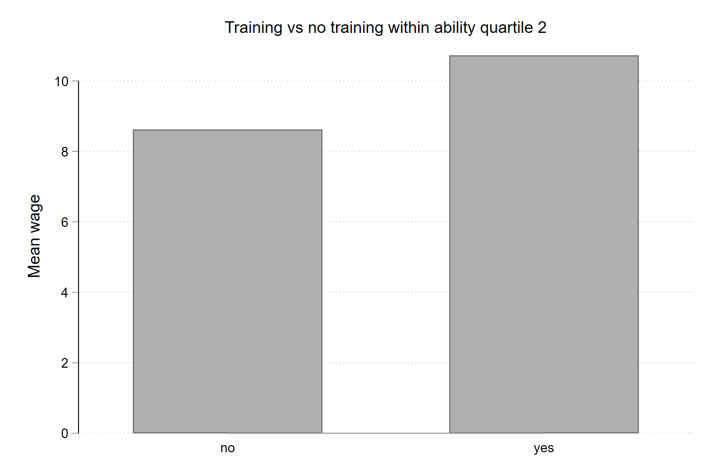
1. Compare wages within quartiles using sum. What is mean wages for each quartile? 2. Using quartile 2 and conditioning on train, what is the conditional mean? How does it compare in size to the true causal effect? 3. Create a simple bar chart of conditional means in that quartile.
RCT vs Observational Study (20 pts)

This exercise builds directly on Exercise 1 and 2. You already created an observational training variable train that is confounded by unobserved ability, and you saw how conditioning on ability reduces bias. Now you will create a randomized version of the training assignment inside the same dataset, generate the corresponding RCT outcome, and compare the naive estimates from the observational data.

Before starting this exercise, you should have the dataset in memory from Exercises 1 and 2 that includes: ability, p_train, train, eps, wage_lat, wage, and ability_q4. If you don’t, re-run your .do file so that it runs Exercises 1 and 2 first.

Start by adding an RCT treatment assignment to your existing data. To make the comparison clean, we will set the RCT treatment probability to match the observed training rate in your observational data. To do this:
- Use egen to compute the share trained individuals in the observational data: p_rct = mean(train)
- Create a variable (u_rct) and is a random variable with a uniform distribution (runiform())
- Create train_rct so that it takes a value of 1 if the value of u_rct is below the value of p_rct (the mean training value in the observational data) and 0 if u_rct is greater than p_rct
- Add variable and value labels
Now, generate the RCT outcome using the same outcome model. Keep the same structural outcome equation you used in Exercise 1, but swap in train_rct:
- wage_rct_lat = 10 + 2*train_rct + 4*ability + eps
- wage_rct = max(wage_rct_lat, 0)
- Add variable labels so your output is easy to read.
1. Compare naive differences in means: observational vs RCT
- Observational estimate (you did this in Exercise 1): $E[wage \mid train=1] - E[wage \mid train=0]$
- RCT estimate: $E[wage_rct \mid train_rct=1] - E[wage_rct \mid train_rct=0]$
Use sum, meanonly, use r() to store group means as scalar, and display the differences with a formatted display statement. What is the naive mean in the observational data, in the rct data, and what is the true causal effect size (again, some of these you have already calculated or know)?

2. Show why the observational estimate is biased by demonstrating selection in the observational data (i.e., ability differs by training status). If there is no selection, mean values should be close to 0 adn the differences in ability by training should also be close to zero. Use tabstat (recommended) or summarize with if. 1. What is mean ability by train? 2. What is the difference in mean ability by train? 3. What is mean ability by train_rct? 4. What is the difference in mean ability by train_rct?
Drawing DAGs for Simple DGPs (10 pts)

For each of the following stories add a comment-only section in your .do file.

1. You want the causal effect of training on wages. Higher-ability workers are more likely to enroll in training, and ability also raises wages. So trained workers earn more partly because of training and partly because they have higher ability. What is the causal effect of training on wages?
1. Draw DAGs using <- ->.
2. Identify confounders (if any), colliders (if any), and mediators (if any).
3. State which variable(s) you would condition on to identify the a causal effect.
2. You want the causal effect of training on wages. Training increases productivity, and productivity increases wages. So training can raise wages directly and also indirectly by raising productivity. What is the causal effect of training on wages?
1. Draw DAGs using <- ->.
2. Identify confounders (if any), colliders (if any), and mediators (if any).
3. State which variable(s) you would condition on to identify the a causal effect.
3. You want the causal effect of training on wages. You’ve collected data on people who are employed. Both training and wages affect whether someone is employed. What is the causal effect of training on wages?
1. Draw DAGs using <- ->.
2. Identify confounders (if any), colliders (if any), and mediators (if any).
3. State which variable(s) you would condition on to identify the a causal effect.

Confounding and Conditional Means (10 pts)

Story: You want the causal effect of training on wages. Higher-ability workers are more likely to enroll in training, and ability also raises wages. So trained workers earn more partly because of training and partly because they have higher ability. What is the causal effect of training on wages?

Copy the following code into your .do file:

* simulate confounding dgp
	clear		all
	set		seed 314159
	set		obs 25000

* confounder
	gen		ability = rnormal(0, 1)

* training selection depends on ability (different rule than earlier exercise)
	gen		p_train = invlogit(-0.5 + 0.8*ability)
	gen		train = (runiform() < p_train)

* wage equation with noise (different levels and effect sizes than earlier exercise)
	gen		eps = rnormal(0, 4)
	gen		wage_lat = 20 + 3.5*train + 6*ability + eps
	gen		wage = max(wage_lat, 0)
	drop		wage_lat

* labels
	lab var		ability "ability (confounder)"
	lab var		p_train "p(train=1)"
	lab var		train "training (selected, not randomized)"
	lab var		eps "wage shock"
	lab var		wage "wage"

	lab def		yesno 0 "no" 1 "yes", replace
	lab val		train yesno

1. What is the true causal effect of training on wages?

2. What is the naive difference in means (confounded)?

Compute the difference in mean wage by train

3. What is the mean of ability with and without training (show selection)?

Report mean ability by train

4. What is are the conditional differences in means (conditioning)?

Create ability_q4 using xtile
Report the differences in mean wage by train for the 3rd ability quartile

Collider Bias Simulation (10 pts)

Story: You want the causal effect of training on wages. You’ve collected data on people who are employed. Both training and wages affect whether someone is employed. What is the causal effect of training on wages?

Copy the following code into your .do file:
```
* simulate collider dgp
	clear		all
	set		seed 24684
	set		obs 50000

* train and wage are independent in the population
	gen		train = (runiform() < 0.5)
	gen		wage  = rnormal(0, 1)

* collider: inclusion depends on both train and wage
	gen		emp_lat = -0.3 + 0.7*train + 0.7*wage + rnormal(0, 1)
	gen		employed = (emp_lat > 0)

* labels
	lab var		train "training (randomized)"
	lab var		wage "wage (independent of training in population)"
	lab var		employed "observed in sample (collider)"

	lab def		yesno 0 "no" 1 "yes", replace
	lab val		train yesno
	lab val		employed yesno
```
1. What is the true causal effect of training on wages?

2. What is the naive difference in mean wages by training status among the employed?
- Compute the difference in mean wage by train using only observations with employed == 1
3. What is the mean probability of being employed with and without training (selection on employment)?
- Report the mean of employed by train
4. What is the difference in mean wages by training status in the full sample (unconditional)?
- Report the difference in mean wage by train using the full dataset
Mediation and Conditional Means (10 pts)

Story: You want the causal effect of training on wages. Training increases productivity, and productivity increases wages. So training can raise wages directly and also indirectly by raising productivity. What is the causal effect of training on wages?

Copy the following code into your .do file:
```
* simulate mediation dgp
	clear		all
	set		seed 13579
	set		obs 50000

* randomized training
	gen		train = (runiform() < 0.5)

* mediator: productivity increases with training
	gen		u_p = rnormal(0, 2)
	gen		productivity = 5 + 1.2*train + u_p

* outcome: wage depends on training directly and indirectly via productivity
	gen		u_w = rnormal(0, 5)
	gen		wage_lat = 25 + 1.0*train + 2.5*productivity + u_w
	gen		wage = max(wage_lat, 0)
	drop		wage_lat

* labels
	lab var		train "training (randomized)"
	lab var		productivity "productivity (mediator)"
	lab var		wage "wage"

	lab def		yesno 0 "no" 1 "yes", replace
	lab val		train yesno
```
1. What is the true direct causal effect of training on wages?

2. What is the naive difference in mean wages by training status (total effect)?
- Compute the difference in mean wage by train
- Save this value (the difference) as a scalar called total_hat
3. What is the indirect effect of training on wages through productivity?
- Compute the difference in mean productivity by train
- Save this value (the difference) as a scalar called delta_p
- Calculate the indirect effect as 2.5*delta_p (from the DGP)
- Save this value as a scalar called indirect_hat
4. What is the implied true direct effect once you subtract off the indirect effect from the total effect?
- Report the direct effect as direct = total − indirect
Check That Your Code Runs (10 pts)

Sometimes you think you’re code runs, but it only actually works because of something else you did previously. To make sure it actually runs you should save your work and then run it in a clean environment.

Follow these steps in to make sure your code really runs:
1. Restart Stata by closing the instance of Stata that you have open.
2. When you reopen Stata, type in the command line clear all. Or, better yet, put clear all at the top of your .do file, after the preamble but before any commands.
3. Rerun your entire homework assignment by clicking the Execute button to make sure it runs from start to finish and produces the expected results.
4. Make sure that you saved your code with the name of the assignment number (i.e., assignment_01). You should see the file in your git repo on your machine.
5. Make sure that your code will run on other computers (relevant for all assignments after the first assignment)
  - No cd. Use a project.do file instead to set directories
  - Use only relative paths in files other than the project.do file
  - Use / not \ for paths
Challenge 8 (Challenge - 20 pts)

In this challenge you will simulate one data generating process (DGP) that contains:
- a confounder (ability) that affects both training and wages
- a mediator (productivity) on the path from training to wages
- a collider (employed) that depends on both training and wages Your job is to use difference-in-means and conditional means (no regressions) to diagnose the bias created by each structure and show how to recover the target causal effect(s).
Copy the following code into your .do file:
```
* simulate one dgp with confounding + mediation + selection
	clear		all
	set		seed 80808
	set		obs 80000

* confounder
	gen		ability = rnormal(0, 1)

* training selection depends on ability (confounding)
	gen		p_train = invlogit(-0.3 + 0.9*ability)
	gen		train = (runiform() < p_train)

* mediator: productivity increases with training and ability
	gen		u_p = rnormal(0, 2)
	gen		productivity = 10 + 1.5*train + 1.0*ability + u_p

* outcome: wage depends on training (direct), productivity (indirect), and ability
	gen		u_w = rnormal(0, 6)
	gen		wage_lat = 30 + 1.2*train + 1.8*productivity + 2.0*ability + u_w
	gen		wage = max(wage_lat, 0)
	drop		wage_lat

* collider: employed depends on training and wage
	gen		emp_lat = -1.0 + 0.6*train + 0.05*wage + rnormal(0, 1)
	gen		employed = (emp_lat > 0)
	drop		emp_lat

* labels
	lab var		ability "ability (confounder)"
	lab var		p_train "p(train=1)"
	lab var		train "training (selected)"
	lab var		productivity "productivity (mediator)"
	lab var		wage "wage"
	lab var		employed "employed (collider / sample selection)"

	lab def		yesno 0 "no" 1 "yes", replace
	lab val		train yesno
	lab val		employed yesno
```
1. True effects from the DGP (do this in comments)
- true direct effect of train on wage
- true indirect effect of train on wage through productivity
- true total effect (= direct + indirect)
(Hint: use the coefficients in the equations above.)

2. Confounding: naive vs conditioned
- Compute the naive difference in mean wages by training status (full sample).
- Show selection by reporting mean ability by training status.
- Reduce confounding by:
  - creating ability_q4 using xtile
  - reporting the difference in mean wage by training within ability quartile 3
3. Collider bias: what changes when you condition on employment?
- Compute the difference in mean wages by training among the employed (employed == 1).
- Report the mean probability of being employed by training status.
- Compare your employed-sample wage difference to the full-sample wage difference from Task 2.
- In comments, explain why conditioning on employed changes the estimate in this DGP.
4. Mediation: total vs indirect vs implied direct (no regressions)
- Using the full sample (do not restrict to employed), compute:
  - total_hat: difference in mean wage by training
- Compute:
  - delta_p: difference in mean productivity by training
  - indirect_hat = 1.8 * delta_p (use the productivity slope from the wage equation)
- Compute:
  - direct_hat = total_hat - indirect_hat
- Compare direct_hat to the true direct effect you wrote in Task 1.

Assignment submission checklist

Assignment