Producing Results

Learning Objectives

Following this assignment students should be able to:

Write formatted text and math equations in LaTeX

Include Stata-produced figures and tables in a LaTeX document

Create coefficient plots with coefplot

Build specification charts for robustness analysis

Produce publication-ready regression and summary statistics tables with esttab

Reading

Topics

LaTeX
Descriptive statistics in tables
Regression results in tables
Regression results as graphics

Readings

Learn LaTeX in 30 minutes by Overleaf
Making regression tables simplified by Ben Jann (The Stata Journal, 2007)
Using Graphs Instead of Tables in Political Science by Kastellec & Leoni (Perspectives on Politics, 2007)

Lecture Notes

Exercises

LaTeX Formatting and Math (10 pts)

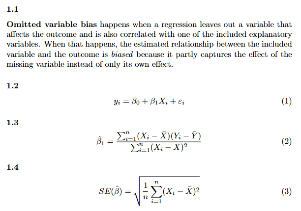
In your lastname.tex file in the semester26 Overleaf project, under \section*{Assignment 10}, write the following using proper LaTeX formatting. You do not need to run any Stata code for this exercise.

1. Write a short paragraph (2–3 sentences) explaining what omitted variable bias is. Bold the term “omitted variable bias” and italicize the word “biased.”

2. Write the OLS regression equation in display math (using \begin{equation} … \end{equation}):

[Y_i = \beta_0 + \beta_1 X_i + \varepsilon_i]

Use \beta, subscripts (_), and \varepsilon.

3. Write the formula for the OLS estimator of $\hat{\beta}_1$ as a displayed equation:

[\hat{\beta}1 = \frac{\sum{i=1}^{n}(X_i - \bar{X})(Y_i - \bar{Y})}{\sum_{i=1}^{n}(X_i - \bar{X})^2}]

Use \hat{}, \bar{}, \frac{}{}, \sum_{i=1}^{n}, and superscripts (^).

4. Write the formula for the standard error of the regression as a displayed equation:

[SE(\hat{\beta}) = \sqrt{\frac{1}{n} \sum_{i=1}^{n} (X_i - \bar{X})^2}]

Use \sqrt{}, \frac{}{}, \sum_{i=1}^{n}, \bar{}, and \hat{}.
Inserting a Stata Figure (10 pts)

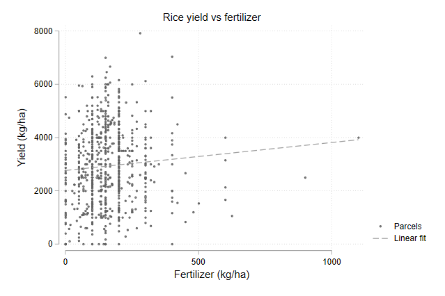
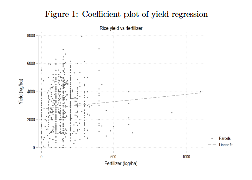
Using tenuredata.dta, create a graph in Stata and include it in your LaTeX document. Start by loading tenuredata.dta.
1. Create a scatter plot of yield against q_f_ha (fertilizer per hectare) with a fitted line (lfit). Choose formatting option for the markers, line, and axis titles.
2. In your lastname.tex under Assignment 10, include the graph. Give it the caption Rice yield vs fertilizer application and label it fig:scatter_rice.

Basic `esttab` Table (10 pts)

Using tenuredata.dta, produce a formatted regression table.

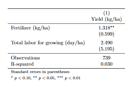
1. In your lastname.tex, include the table using \input{10-rice-regs.tex} inside a table environment.

Run reg yield q_f_ha lt_f_ha, vce(cluster panelid) a
Store results as r1.

Display the table with esttab:

 esttab      r1 using "$answ/10-esttab-basic-1.tex", replace ///
                 se star(* 0.10 ** 0.05 *** 0.01) ///
                 keep(q_f_ha lt_f_ha) ///
                 label booktabs ///
                 stats(N r2, labels("Observations" "R-squared") fmt(0 3))

In your lastname.tex, include the table using \input{10-esttab-basic-1.tex} inside a table environment.

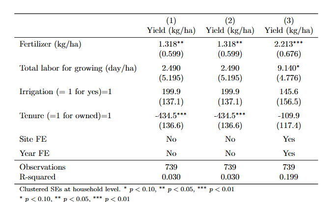
2.Run and store three regressions, all with vce(cluster panelid):

r2: yield on q_f_ha lt_f_ha i.irrig i.tenure
r3: yield on q_f_ha lt_f_ha i.irrig i.tenure i.site i.year
Display a three-column table with esttab and export it to LaTeX:

   esttab      r1 r2 r3 using "$answ/10-esttab-basic-2.tex", replace ///
                   se star(* 0.10 ** 0.05 *** 0.01) ///
                   keep(q_f_ha lt_f_ha 1.irrig 1.tenure) ///
                   order(q_f_ha lt_f_ha 1.irrig 1.tenure) ///
                   label booktabs ///
                   indicate("Site FE = *.site" "Year FE = *.year") ///
                   stats(N r2, labels("Observations" "R-squared") fmt(0 3)) ///
                   note("Clustered SEs at household level." ///
                        "\sym{*} \(p<0.10\), \sym{**} \(p<0.05\), " ///
                        "\sym{***} \(p<0.01\)")

In your lastname.tex, include the table using \input{10-esttab-basic-2.tex} inside a table environment.

Multi-Column Table with Notes (20 pts)

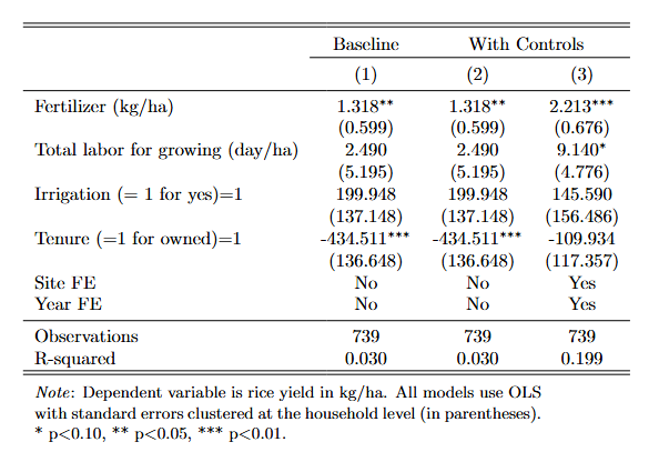
Using tenuredata.dta (rice observations only), produce a multi-column regression table and export it to LaTeX. Run and store three regressions, all with vce(cluster panelid):

r1: yield on q_f_ha lt_f_ha
r2: yield on q_f_ha lt_f_ha i.irrig i.tenure
r3: yield on q_f_ha lt_f_ha i.irrig i.tenure i.site i.year

Display a three-column table with esttab and export it to LaTeX using the prehead, postfoot, and fragment options to create grouped column headers and a detailed note:

   esttab      r1 r2 r3 using "$answ/10-rice-regs.tex", replace ///
                   b(3) se(3) ///
                   keep(q_f_ha lt_f_ha 1.irrig 1.tenure) ///
                   order(q_f_ha lt_f_ha 1.irrig 1.tenure) ///
                   star(* 0.10 ** 0.05 *** 0.01) ///
                   indicate("Site FE = *.site" "Year FE = *.year") ///
                   stats(N r2, labels("Observations" "R-squared") fmt(0 3)) ///
                   noobs booktabs nonum nomtitle collabels(none) ///
                   nobaselevels nogaps fragment label ///
                   prehead("\begin{tabular}{l*{3}{c}} " ///
                     "\\[-1.8ex]\hline \hline \\[-1.8ex] " ///
                     "& \multicolumn{1}{c}{Baseline} & " ///
                     "\multicolumn{2}{c}{With Controls} \\ " ///
                     "\cline{2-2} \cline{3-4} \\[-1.8ex] " ///
                     "& \multicolumn{1}{c}{(1)} & " ///
                     "\multicolumn{1}{c}{(2)} " ///
                     "& \multicolumn{1}{c}{(3)} \\ \midrule") ///
                   postfoot("\hline \hline \\[-1.8ex] " ///
                     "\multicolumn{4}{p{0.8\linewidth}}{\small " ///
                     "\noindent \textit{Note}: Dependent variable " ///
                     "is rice yield in kg/ha. All models use " ///
                     "OLS with standard errors clustered at the " ///
                     "household level (in parentheses). " ///
                     "* p$<$0.10, ** p$<$0.05, *** p$<$0.01.} " ///
                     "\end{tabular}")

In your lastname.tex, include the table using \input{10-rice-regs.tex} inside a table environment. To get the *** to render correctly, you’ll need to add \def\sym#1{\ifmmode^{#1}\else$^{#1}$\fi} to your preamble.

Summary Statistics Table (10 pts)

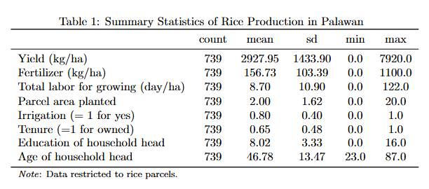
Using tenuredata.dta (rice observations only), produce a summary statistics table.
- First, run estimates clear to clear any previously stored estimates.
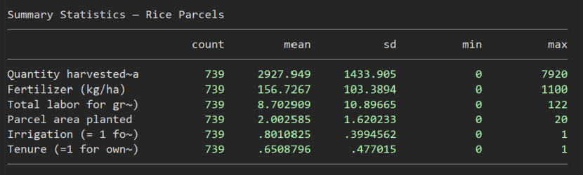
- Use estpost sum to compute summary statistics for: yield, q_f_ha, lt_f_ha, area, irrig, tenure.
- Display the table with:
```
 esttab,     cells("count mean sd min max") ///
                 noobs nonumber nomtitle ///
                 title("Summary Statistics — Rice Parcels") ///
                 label
```
Basic `coefplot` (10 pts)

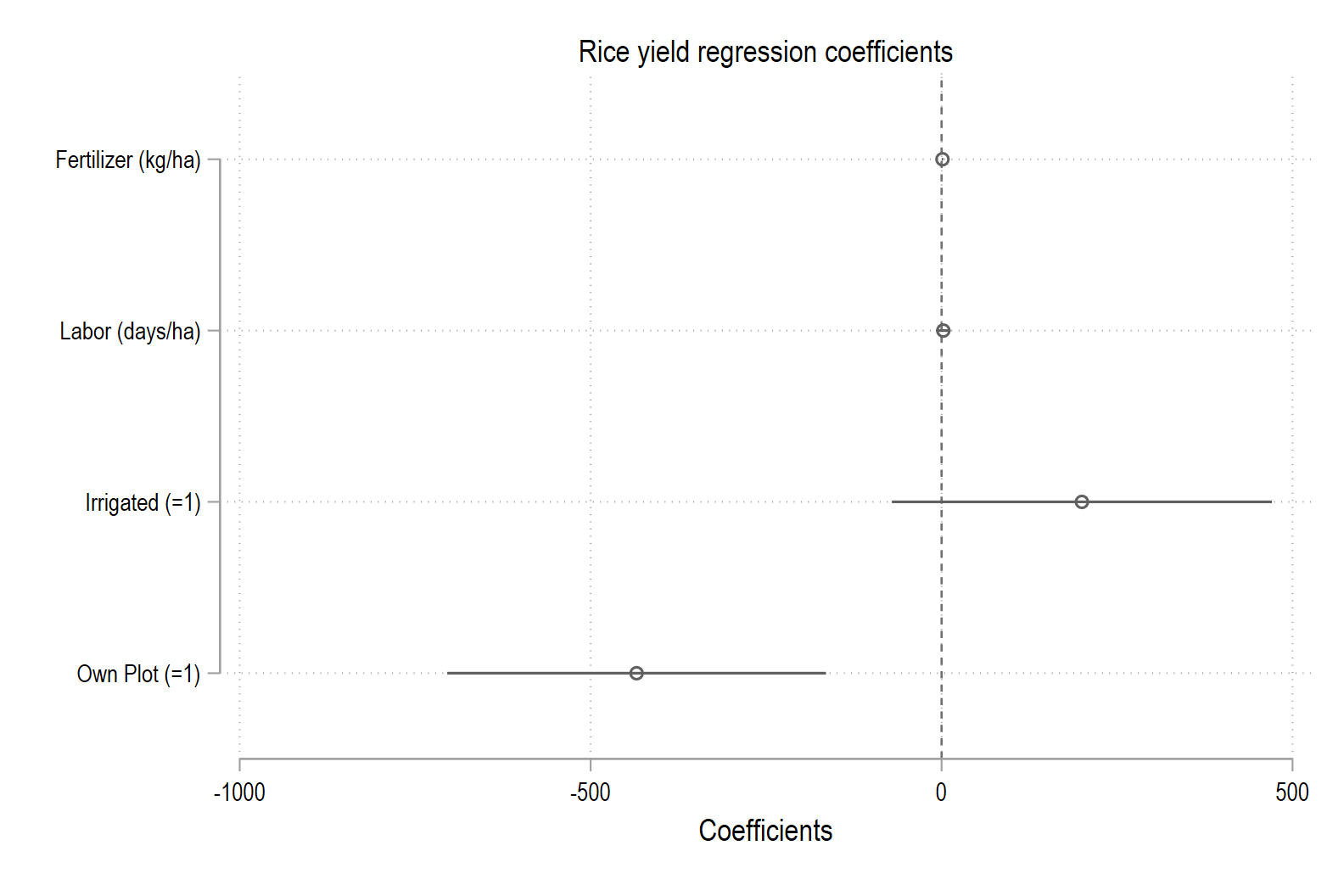
Using tenuredata.dta, create a coefficient plot.
- Run a regression of yield on q_f_ha, lt_f_ha, i.irrig, and i.tenure, with standard errors clustered at the household level: vce(cluster panelid).
- Create a coefficient plot using coefplot:
  - Drop the constant (drop(_cons))
  - Add a vertical reference line at zero (xline(0))
  - Relabel the coefficients to be more descriptive
  - Add a title and an xtitle
- Export the graph: graph export "$answ/10-coefplot-basic.png", replace
Multi-Model `coefplot` (10 pts)

Using tenuredata.dta, compare the fertilizer and labor coefficients across multiple specifications.
- Run and store three regressions, all with vce(cluster panelid):
  - m1: yield on q_f_ha lt_f_ha i.irrig i.tenure
  - m2: yield on q_f_ha lt_f_ha i.irrig i.tenure i.site
  - m3: yield on q_f_ha lt_f_ha i.irrig i.tenure i.site i.year
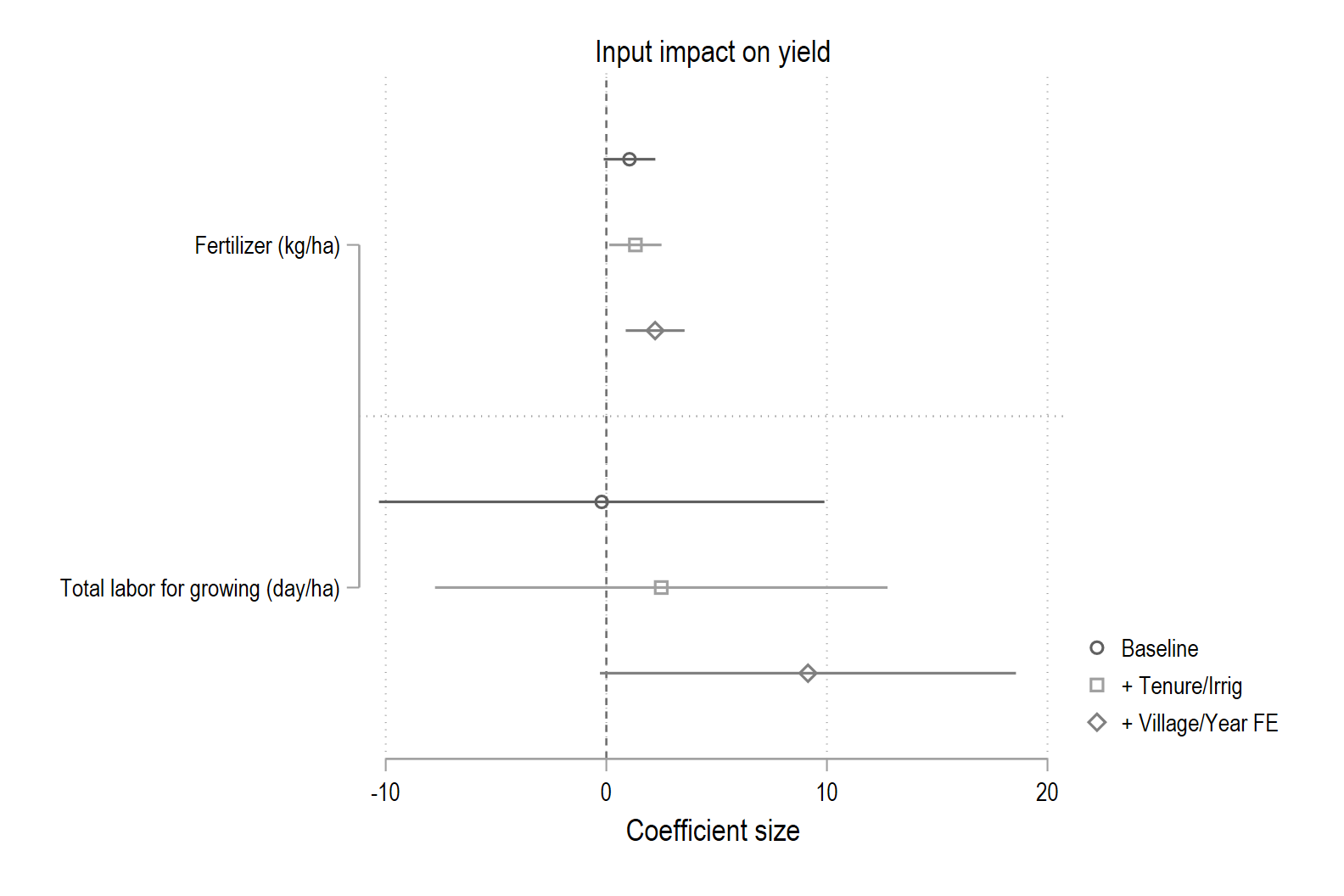
- Create a multi-model coefplot showing only q_f_ha and lt_f_ha:
```
 coefplot    (m1, label("Baseline") ) ///
             (m2, label("+ Tenure/Irrig") ) ///
             (m3, label("+ Village/Year FE") ), ///
                keep(q_f_ha lt_f_ha) xline(0) ///
                xtitle("Coefficient size")
```
- Export the graph: graph export "$answ/10-coefplot-multi.png", replace
- In your lastname.tex, include the graph using \includegraphics[width=0.8\textwidth]{10-coefplot-multi.png}
Specification Chart (15 pts)

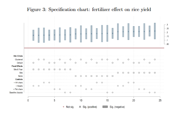
Using tenuredata.dta, build a specification chart that shows how the fertilizer coefficient varies across many specifications. You can do this by adapting the code from the lecture notes, replacing variable names and labels as necessary.
- Use postfile to loop over specifications varying the controls, fixed effects, and standard errors (use lny as the dependent variable):
  - Controls (4 levels): (1) baseline (lnf lnl lnp), (2) + plot characteristics (i.irrig i.tenure), (3) + assets (tractor carabao), (4) + HH characteristics (hhsize educhoh agehoh)
  - Fixed Effects (3 levels): (1) none, (2) site (i.site), (3) site and year (i.site i.year)
  - Standard errors (2 levels): (1) default, (2) clustered at panelid
- Store the coefficient on lnf, its SE, and the 95% CI from each specification.
- After the loop, load the results and create significance indicators:
- Sort by beta and generate obs = _n.
- Stack specification indicators for the bottom panel (controls, FEs, SEs) and adjust your dual y-axis plot to match the 24 regressions and the new categories. Use colors to distinguish significant positive (blue), significant negative (maroon), and not significant (black) results.
- Export: graph export "$answ/10-spec-chart-rice.png", replace
- In your lastname.tex, include the graph using \includegraphics[width=0.8\textwidth]{10-spec-chart-rice.png}
Check That Your Code Runs (5 pts)

Sometimes you think you’re code runs, but it only actually works because of something else you did previously. To make sure it actually runs you should save your work and then run it in a clean environment.

Follow these steps in to make sure your code really runs:
1. Restart Stata by closing the instance of Stata that you have open.
2. When you reopen Stata, type in the command line clear all. Or, better yet, put clear all at the top of your .do file, after the preamble but before any commands.
3. Rerun your entire homework assignment by clicking the Execute button to make sure it runs from start to finish and produces the expected results.
4. Make sure that you saved your code with the name of the assignment number (i.e., assignment_01). You should see the file in your git repo on your machine.
5. Make sure that your code will run on other computers (relevant for all assignments after the first assignment)
  - No cd. Use a project.do file instead to set directories
  - Use only relative paths in files other than the project.do file
  - Use / not \ for paths
Challenge 10 (Challenge - 20 pts)

This challenge uses tenuredata.dta to practice skills from all three lectures (LaTeX, coefplot, estout). You will produce a short results section with a summary statistics table and a coefficient plot — all integrated into your LaTeX document. Reload the tenuredata.dta and type estimates clear.

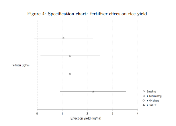
1. Use estpost sum to compute summary statistics for: yield, q_f_ha, lt_f_ha, area, irrig, tenure, educhoh, aghoh. Then export the table to $answ/10-challenge-sumstats.tex using esttab with booktabs and label, posthead, postfoot, nonum, nomtitle, nobaselevels, nogaps, and fragment.

2. Create a multi-model coefplot comparing q_f_ha across the four regressions with vce(cluster panelid). Then export: graph export "$answ/10-challenge-coefplot.png", replace
- c1: yield on q_f_ha lt_f_ha
- c2: yield on q_f_ha lt_f_ha i.irrig i.tenure
- c3: yield on q_f_ha lt_f_ha i.irrig i.tenure educhoh agehoh
- c4: yield on q_f_ha lt_f_ha i.irrig i.tenure educhoh agehoh i.site i.year
3. In your lastname.tex under Assignment 10, create a short results section that includes:
- A couple sentences discuss the summary statistics table and referencing the table (use \ref{})
- The summary statistics table (\input{10-challenge-sumstats.tex}) with a title using \caption{} and label using \label{}
- A couple sentences discuss the coefficient plot and referencing the figure (use \ref{})
- The coefficient plot (\includegraphics{10-challenge-coefplot.png}) with a title using \caption{} and label using \label{}
- Compile and verify everything renders correctly.

Assignment submission checklist

Assignment