Learning Objectives
Following this assignment students should be able to:
- Implement first differencing and demeaning manually
- Run one-way fixed effects using LSDV,
xtreg, andreghdfe- Identify the staggered adoption problem in TWFE
- Use modern TWFE estimators such as
csdid
Reading
Topics
- How fixed effects work
- Individual intercepts
- First differencing
- De-meaning
- Two-way fixed effects
-
Clustered standard errors
- Reading (chapter 16): The Effect
Additional Suggested Readings (Recent TWFE Literature)
The literature on Two-Way Fixed Effects (TWFE) and staggered treatment adoption has evolved rapidly. To understand the issues with standard TWFE and modern estimators, see:
- The Problem: Goodman-Bacon, A. (2021). “Difference-in-differences with variation in treatment timing.” Journal of Econometrics.
- A Solution: Callaway, B., and Sant’Anna, P. H. (2021). “Difference-in-differences with multiple time periods.” Journal of Econometrics.
- Accessible Overview: Baker, A. C., Larcker, D. F., and Wang, C. C. (2022). “How much should we trust staggered difference-in-differences estimates?” Journal of Financial Economics.
Lecture Notes
Exercises
-
First Differencing (20 pts)
We will use the
mm.dtadataset for these exercises. Recall that it is a panel dataset tracking agricultural households in Ethiopia over time. The panel identifier isqnno(household) and the time identifier istindex(time index).- Load
mm.dta. - Start by running a pooled OLS regression of
yieldontotfertcostha, clustering the standard errors at theqnnolevel. - Sort the dataset by the panel identifier (
qnno) and the time variable (tindex). - Generate a first-differenced variable for yield
d_yield(e.g.,yield - yield[_n-1]) byqnno. - Generate a first-differenced variable for fertilizer input
d_fert(e.g.,totfertcostha - totfertcostha[_n-1]) byqnno. - Run a regression of the differenced yield on the differenced fertilizer variable, clustering the standard errors at the
qnnolevel.
1. Use
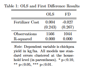
eststoto save the pooled OLS and FD results. Then useesttabto create a table of results using the following table structure:esttab ols fd using "$answ/11-fd.tex", replace /// b(3) se(3) /// rename(totfertcostha "Fertilizer Cost" d_fert "Fertilizer Cost") /// keep("Fertilizer Cost") /// star(* 0.10 ** 0.05 *** 0.01) /// stats(N r2, labels("Observations" "R-squared") fmt(0 3)) /// noobs booktabs nonum nomtitle collabels(none) /// nobaselevels nogaps fragment label /// prehead("\begin{tabular}{l*{2}{c}} " /// "\\[-1.8ex]\hline \hline \\[-1.8ex] " /// "& \multicolumn{1}{c}{OLS} & " /// "\multicolumn{1}{c}{FD} \\ \midrule") /// postfoot("\hline \hline \\[-1.8ex] " /// "\multicolumn{3}{p{\linewidth}}{\small " /// "\noindent \textit{Note}: Dependent variable " /// "is chickpea yield in kg/ha. All models use " /// "standard errors clustered at the " /// "household level (in parentheses). " /// "* p$<$0.10, ** p$<$0.05, *** p$<$0.01.} " /// "\end{tabular}")2. What is the effect of a change in fertilizer cost on chickpea yield? How does it compare to the pooled OLS estimate?
- Load
-
Demeaning the Data (10 pts)
Using
mm.dta:- Use
egenwithbysort qnno:to calculate the household-specific mean foryield. - Do the same to calculate the household-specific mean for fertilizer cost
totfertcostha. - Generate demeaned versions of both variables by subtracting the household mean from the original value (e.g.,
dm_yieldanddm_fert). - Run a regression of the demeaned yield on the demeaned fertilizer, clustering standard errors by
qnno.
- Use
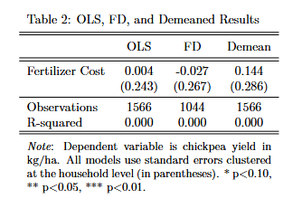
eststoto save the demeaned results. Then adapt the table structure from the previous exercise to create a table of results with a third column headedDemean. - What is the coefficient on fertilizer cost in the demeaned regression and how does it compare to the coefficients you calculated in Exercises 1?
- Use
-
Dummy Variables (10 pts)
Using
tenuredata.dta(restricted torice == 1):- Instead of manually demeaning the data, use the
i.operator to include a fixed effect dummy for every individual household (panelid). - Run a regression of raw
yieldonq_f_haand your dummy variables (i.panelid). Cluster the standard errors bypanelid.
Does the regression even run on your version of Stata? If so,
- Use
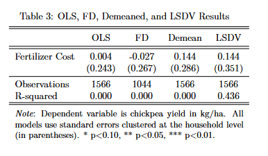
eststoto save the LSDV results. Then adapt the table structure from the previous exercise to create a table of results with a fourth column headedLSDV. - What is the coefficient on fertilizer in the LSDV regression and how does it compare to the coefficients you calculated in Exercises 1 and 2?
- Instead of manually demeaning the data, use the
-
Using `xtreg` (10 pts)
Using
mm.dta:- Tell Stata that your dataset is a panel using the
xtsetcommand. Specifyqnno tindexas the panel identifiers. - Run a fixed effects regression of
yieldontotfertcosthausing thextregcommand with the, feoption. Cluster standard errors at theqnnolevel.
- Use
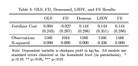
eststoto save the FE results. Then adapt the table structure from the previous exercise to create a table of results with a fifth column headedFE. - What is the coefficient on fertilizer cost in the FE regression and how does it compare to the coefficients you calculated in Exercises 1-3?
- Tell Stata that your dataset is a panel using the
-
Adding Time Fixed Effects (10 pts)
Using
mm.dta, let’s extend our models from the One-Way FE lecture.- Ensure your data is
xtset qnno tindex. - Run a standard One-Way Fixed Effects model. Regress
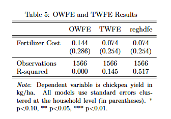
yieldon fertilizer cost (totfertcostha) usingxtreg, fe. Cluster standard errors at theqnnolevel. - Run a standard Two-Way Fixed Effects model. Regress
yieldon fertilizer cost (totfertcostha) usingxtreg, fe, but this time include time fixed effects by addingi.tindexto your list of covariates. Cluster standard errors at theqnnolevel. - Now estimate the exact same model using the
reghdfecommand. Specifyabsorb(qnno tindex)to absorb both individual and time fixed effects. Cluster standard errors at theqnnolevel.
- Use
eststoto save each of the three results. Then adapt the table structure from the Exercise 1 to create a table of results heading columns withOWFE,TWFE, andreghdfe. - How do the estimates on
totfertcosthacompare across the three models? Did aggregate time shocks bias the one-way fixed effect estimator?
- Ensure your data is
-
Staggered Adoption Cohorts (15 pts)
Using
mm.dta, we want to evaluate the effect of improved chickpea adoption (icp) on yield. However, parcels adopt improved chickpeas at different times. We need to create a variable that stores the first time period a parcel ever hadicp == 1.- Sort the data by
qnnoandtindex. - Create a variable
first_icpthat equalstindexificp == 1, and missing otherwise. - Use
bysort qnno:to replacefirst_icpwith the minimum value offirst_icpfor that parcel across all years (egen ... = min()). - For parcels that never adopted improved chickpeas (
missing(first_icp)), replacefirst_icp= 0.
You now have the exact cohort group variable needed for modern TWFE estimators. Run a TWFE regression using either
xtregwith time dummies (i.tindex) orreghdfeand useeststoto save the result. What is the coefficient on improved chickpea adoption?
- Sort the data by
-
Modern TWFE Estimators (20 pts)
Let’s do a Bacon decomposition and then apply Callaway & Sant’Anna’s modern robust estimator to
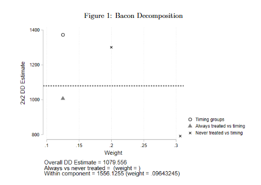
mm.dtausing thefirst_icpcohort variable we just built.- Run
bacondecomp yield icp, ddetail. Save the resulting figure as a.pngfile and import it into yourlastname.texunder Assignment 11. Give it the captionBacon Decompositionand label itfig:bacon. - Now run
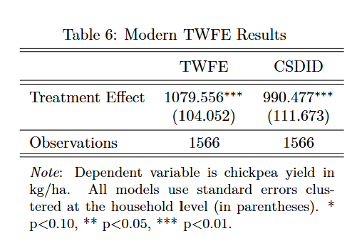
csdid yield, ivar(qnno) time(tindex) gvar(first_icp) tr(icp). Calculate the aggregated overall ATT by runningestat eventand useeststoto save the result. Then useesttabto create a table of the results from this model and the TWFE model you estimated in the last exercise. - How do these results compare to the standard Two-Way Fixed Effects estimate you found in the last exercise?
- Run
-
Check That Your Code Runs (5 pts)
Sometimes you think you’re code runs, but it only actually works because of something else you did previously. To make sure it actually runs you should save your work and then run it in a clean environment.
Follow these steps in to make sure your code really runs:
-
Restart Stata by closing the instance of Stata that you have open.
-
When you reopen Stata, type in the command line
clear all. Or, better yet, putclear allat the top of your.dofile, after the preamble but before any commands. -
Rerun your entire homework assignment by clicking the
Executebutton to make sure it runs from start to finish and produces the expected results. -
Make sure that you saved your code with the name of the assignment number (i.e.,
assignment_01). You should see the file in your git repo on your machine. -
Make sure that your code will run on other computers (relevant for all assignments after the first assignment)
- No
cd. Use aproject.dofile instead to set directories - Use only relative paths in files other than the
project.dofile - Use
/not\for paths
- No
-
-
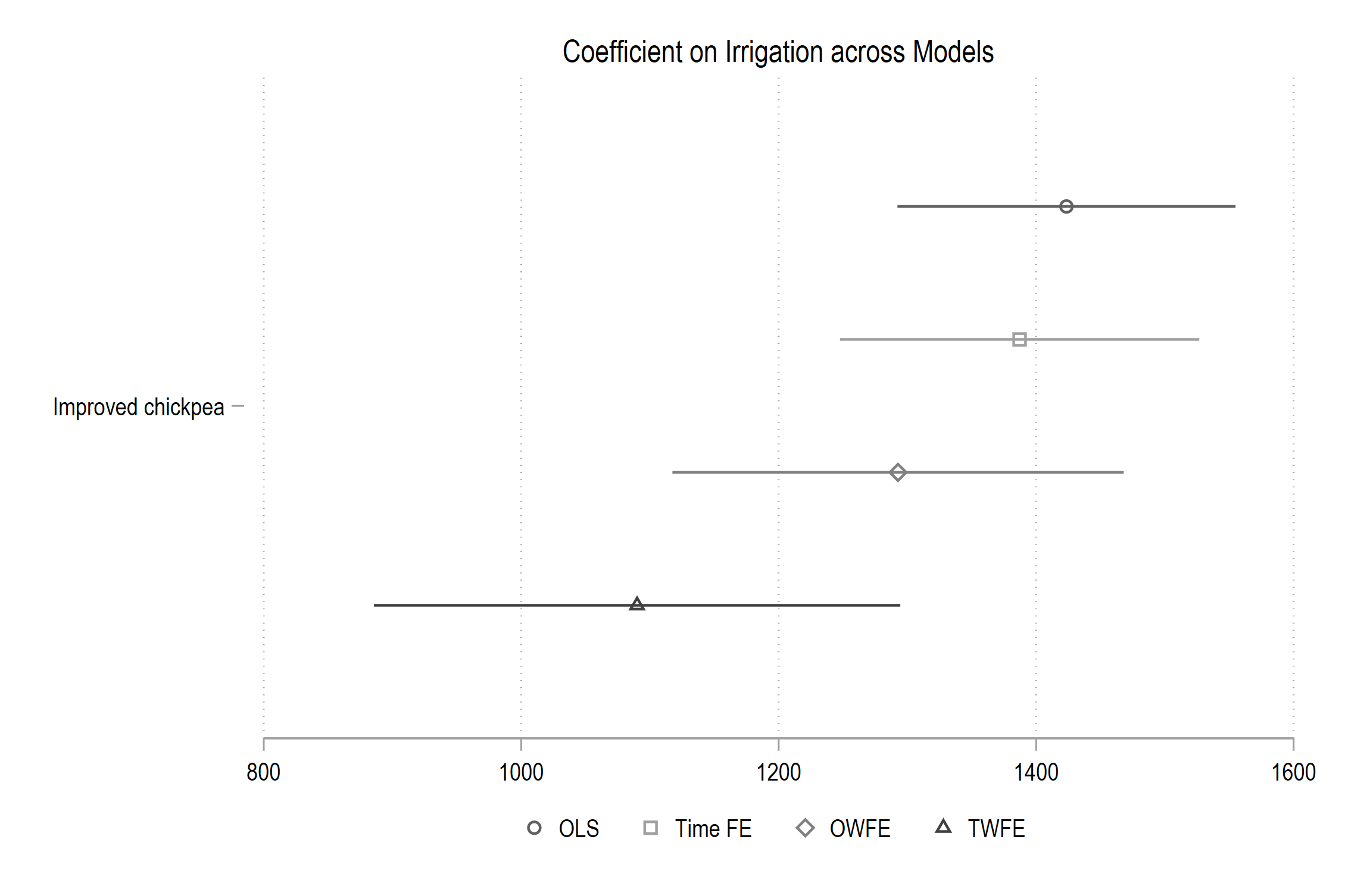
Challenge 11 (Challenge - 20 pts)
This challenge combines everything you’ve learned about Fixed Effects,
estout, andcoefplotto test the sensitivity of theicpcoefficient across multiple Fixed Effect specifications.- Load the
mm.dtadataset. - Run the following four models and store their estimates (e.g.,
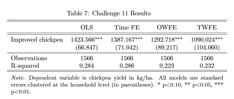
eststo c1, etc.):- Model 1: Pooled OLS (
reg). Regressyieldonicp totfertcostha totchemcostha. - Model 2: Time Fixed Effects (
reg). Addi.tindexto Model 1. - Model 3: One-Way Fixed Effects (
xtreg, fe). Addxtsetand run the model without time dummies. - Model 4: Two-Way Fixed Effects (
xtreg, fe). Addi.tindexto Model 3.
- Model 1: Pooled OLS (
- For all 4 models, cluster the standard errors by
qnno.
- Use
esttabto create a table of the coefficient onicpacross all four models. Adapt the table structure from Week 10, Exercise 4 to create a table of results. In your lastname.tex, include the table using\input{11-challenge-regs.tex}inside a table environment that I provide for Assignment 11 in Overleaf. Give the table a caption and label. - Use
coefplotto graph the coefficient onicpacross all four models. Adapt the figure structure from Week 10, Exercise 7 to create a single figure of results. Add a horizontal line at 0 (xline(0)) and customize the legend to cleanly label the four models. In your lastname.tex, include the graph using\includegraphics[width=0.8\textwidth]{11-challenge-coefplot.png}inside a figure environment. Give the graph a caption and label.
- Load the
Assignment submission checklist
Solutions
- First Differencing 1, 2
- Demeaning the Data 1, 2
- Dummy Variables 1, 2
- Using
xtreg1, 2 - Adding Time Fixed Effects 1, 2
- Staggered Adoption Cohorts
- Modern Estimators 1, 2, 3
- Check That Your Code Runs
- Challenge 11 1, 2