Instrumental Variables · Coding for Applied Economists

Learning Objectives

Following this assignment students should be able to:

Construct instrumental variables regressions

Conduct overidentification and weak instrument tests

Calculate robust standard errors

Estimate bootstraped standard errors

Conduct randomization inference

Apply multiple hypothesis testing corrections

Reading

Topics

Instrumental variables
Two-stage least squares
Weak instruments
Testing for endogeneity
First-stage regressions
Testing for exogeneity

Readings

Reading (chapter 19): The Effect

Lecture Notes

Exercises

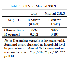
Manual 2SLS (10 pts)

In this week’s exercises, you will be using data from Michler et al. (2019), which studies the impact of conservation agriculture (CA) on crop yields in Zimbabwe. CA adoption (CA) is endogenous — farmers who adopt CA may differ systematically from those who don’t. In the paper, we instrument CA adoption using wardNGO, the number of other households in the same ward that received NGO support for CA.

Load "$data/Michler_JEEM.dta" and keep only maize observations (keep if crop == 1).
Run a naive OLS regression of lnyield on CA with the following controls: lnbasal lntop lnseed lnaream2 pdate pdate2 i.year, clustering standard errors at the rc level. Store the results as ols.
Run the First Stage: Regress the endogenous variable (CA) on the instrument (wardNGO) and all the same controls (lnbasal lntop lnseed lnaream2 pdate pdate2 i.year), clustering at rc. Store as first.
Generate the predicted fitted values from the first stage using predict CA_hat, xb.
Run the Second Stage: Regress lnyield on CA_hat and the same controls, clustering at rc. Store as manual.

1. Export a two-column table comparing OLS and Manual 2SLS and put it in your Overleaf file:

* compare ols and manual 2sls
	esttab      ols manual using "$answ/13-iv-manual.tex", replace ///
	                b(3) se(3) ///
	                keep(CA) rename(CA_hat CA) nodepvars ///
	                star(* 0.10 ** 0.05 *** 0.01) ///
	                nomtitles fmt(0 3)) ///
	                stats(N r2, labels("Observations" "R-squared") /// 
	                noobs booktabs nonum collabels(none) ///
	                nobaselevels nogaps fragment label ///
	                prehead("\begin{tabular}{l*{2}{c}} " ///
	                    "\\[-1.8ex]\hline \hline \\[-1.8ex] " ///
	                    "& \multicolumn{1}{c}{OLS} & " ///
	                    "\multicolumn{1}{c}{Manual 2SLS} " ///
	                    "\\ \midrule") ///
	                postfoot("\hline \hline \\[-1.8ex] " ///
	                    "\multicolumn{3}{p{\linewidth}}{\small " ///
	                    "\noindent \textit{Note}: Dependent var. " ///
	                    "is log maize yield. Standard errors " ///
	                    "clustered at household level in " ///
	                    "parentheses. Manual 2SLS standard errors " ///
	                    "are incorrect. " ///
	                    "* p$<$0.10, ** p$<$0.05, *** p$<$0.01.} " ///
	                    "\end{tabular}")

2. Does the coefficient on CA increase or decrease when you move from OLS to the manual 2SLS? What does this tell you about the direction of the selection bias?

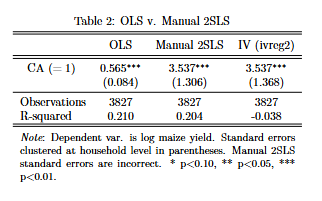
Using `ivreg2` (10 pts)

The manual 2SLS from the previous exercise produces correct coefficients but incorrect standard errors, because Stata doesn’t know that CA_hat is an estimated variable. Now we’ll use the user-written ivreg2 command, which handles both stages simultaneously, properly adjusts the standard errors, and automatically reports key diagnostic statistics (weak instrument F-stat, overidentification test).
- Using Michler_JEEM.dta (maize only), run ivreg2 with wardNGO as the instrument for CA, including the same controls as Exercise 1 (lnbasal lntop lnseed lnaream2 pdate pdate2 i.year) and clustering at rc. Use the first option to display the first-stage results. Store as iv.
1. Adapt the table code from Exercise 1 to add a third column for ivreg2 and export to Overleaf.

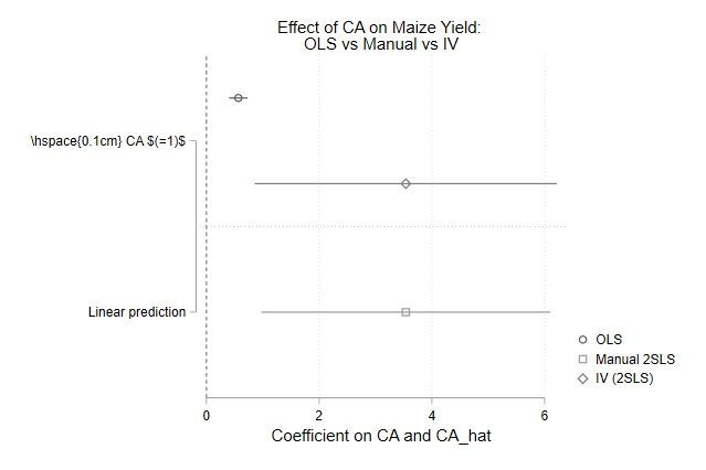
2. Create a coefplot comparing the CA coefficient across OLS, manual 2SLS, and ivreg2 and export to Overleaf:
```
* coefficient plot comparing OLS, Manual, and IV
	coefplot        (ols, label("OLS")) ///
	                (manual, label("Manual 2SLS")) ///
	                (iv, label("IV (2SLS)")), ///
	                    keep(CA CA_hat) xline(0) ///
	                    title("Effect of CA on Maize Yield: " ///
	                    "OLS vs Manual vs IV") ///
	                    xtitle("Coefficient on CA and CA_hat") ///
	                    graphregion(color(white))
	graph export    "$answ/13-iv-coefplot.png", replace
```
3. Is the coefficient on CA from ivreg2 identical to the one you found manually in Exercise 1?

4. Are the standard errors the same? Why or why not?
Panel IV with `xtivreg2` (10 pts)

In the previous exercises we estimated the effect of conservation agriculture on maize yields using cross-sectional IV. But the Michler_JEEM.dta dataset is actually a panel: households (rc) are observed over multiple years. This means we can absorb time-invariant household heterogeneity with fixed effects while instrumenting for CA adoption.

For whatever reason, xtivre2 can’t hand factor-variable operators like i.year. So, before running your regressions, use the Stata command qui tab year, gen(y_) to create dummy variables for each year and include these in your regressions.
- Using Michler_JEEM.dta (maize only), declare the panel structure with xtset rc.
- Run a fixed effects regression using xtreg using the same variables as in the previous exercises but adding feand cluster(rc). Store as fe.
- Run a panel IV regression using xtivreg2 using the same variables as in the previous exercises but adding fe and cluster(rc). Store as fe_iv.
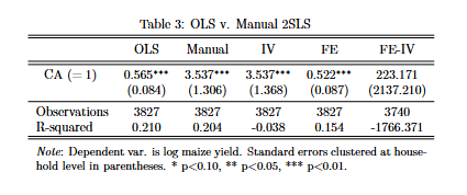
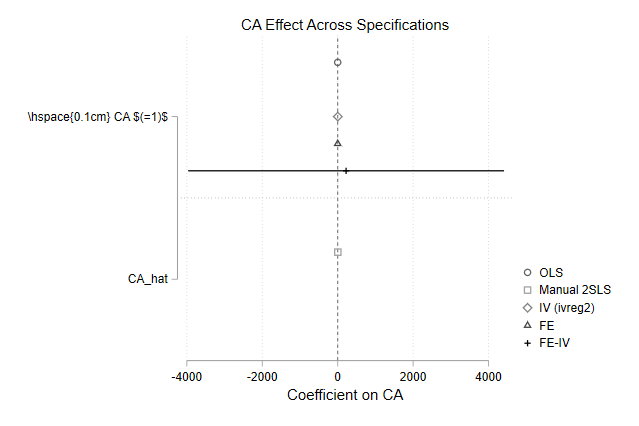
1. Adapt your previous table to add 2 more columns. Order results as ols, manual, iv, fe, fe_iv. Export and put into Overleaf.

2. Adapt your previous coefplot to include all 5 specifications and export to Overleaf.

3. How does the CA coefficient change when you move from pooled OLS to fixed effects? What does this tell you about time-invariant confounders?

4. How does the CA coefficient change when you add IV? What does this tell you about time-varying confounders?
Instrument Diagnostics (10 pts)

Before trusting any IV estimate, we must test whether our instrument is actually valid. In this exercise you will run the standard battery of diagnostic tests on the Michler_JEEM.dta conservation agriculture IV specification.
- Using Michler_JEEM.dta (maize only), run xtivreg2 with clustered standard errors
  - Add the first option to display both first- and second-stage results
  - Add the endog(CA) option to display the Durbin-Wu-Hausman Test
1. Does wardNGO pass the standard rule-of-thumb threshold of $F > 10$ for instrument strength using the Kleibergen-Paap F-statistic?
2. Based on the endogeneity test, is CA statistically endogenous?
3. We have exactly one instrument (wardNGO) for one endogenous variable (CA). What does the Stata output say about the Hansen J-statistic?

Robust & Clustered Standard Errors (10 pts)

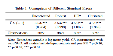
In this exercise you will compare different approaches to calculating standard errors for the conservation agriculture IV regression from Michler_JEEM.dta. The base specification is a pooled IV model using ivreg2 with household fixed effects.

Run the panel IV regression with default (uncorrected) standard errors.
Run the same specification but with the robust option.
The bw(1) kernel(tru) options require the data to be tsset. Since the data has multiple plots per household-year, generate a unique observation ID (gen obs_id = _n) and tsset obs_id before running this specification.
Run the same specification but using the Bell-McCaffrey corrections bw(1) kernel(tru).
Run the same specification but with the standard error option cluster at the household (rc) level.

1. Export a four-column comparison table and put it in your Overleaf file:

* compare standard error methods
	esttab      def robust hc2 cluster ///
	                using "$answ/13-se-hc2.tex", replace ///
	                b(3) se(3) keep(CA) nomtitles ///
	                star(* 0.10 ** 0.05 *** 0.01) ///
	                stats(N, labels("Observations") fmt(0)) ///
	                noobs booktabs nonum collabels(none) ///
	                nobaselevels nogaps fragment label ///
	                prehead("\begin{tabular}{l*{4}{c}} " ///
	                    "\\[-1.8ex]\hline \hline \\[-1.8ex] " ///
	                    "& \multicolumn{1}{c}{Uncorrected} & " ///
	                    "\multicolumn{1}{c}{Robust} & " ///
	                    "\multicolumn{1}{c}{HC2} & " ///
	                    "\multicolumn{1}{c}{Clustered} " ///
	                    "\\ \midrule") ///
	                postfoot("\hline \hline \\[-1.8ex] " ///
	                    "\multicolumn{5}{p{0.9\linewidth}}{\small " ///
	                    "\noindent \textit{Note}: Dependent variable " ///
	                    "is log maize yield. CA instrumented with " ///
	                    "wardNGO. All models include input controls " ///
	                    "and year FE. " ///
	                    "* p$<$0.10, ** p$<$0.05, *** p$<$0.01.} " ///
	                    "\end{tabular}")

1. Compare the standard error on CA across HC1, HC2, and the panel FE specifications. Does adjusting for leverage (HC2) increase or decrease the standard error?

2. How do the clustered standard errors compare to the robust standard errors? What does this suggest about within-household correlation in this panel?

Bootstrap Comparisons (10 pts)

If we aren’t satisfied with analytical approximations of standard errors, we can calculate them empirically through bootstrapping. In this exercise you will compare bootstrap standard errors to the analytical standard errors from the previous exercise.
- Using Michler_JEEM.dta (maize only), run the pooled IV regression (ivreg2) with bootstrap standard errors.
- Set the seed to 5453654.
- Bootstrap the regression 1,000 times.
- Cluster the standard errors at the household (rc) level.
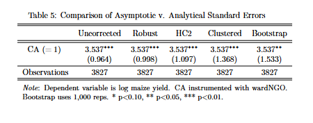
1. Adapt the table code from Exercise 1 to add a fifth column for the bootstrap results and export to Overleaf.
2. Are the bootstrapped standard errors closer to the robust or the clustered standard errors from the previous exercise?
Wild Cluster Bootstrap (10 pts)

Clustered standard errors rely on asymptotic theory and require a large number of independent clusters (typically 42+) to be reliable. In this exercise you will test what happens when you cluster at a level with relatively few clusters, and then correct using the Wild Cluster Bootstrap.
- Using Michler_JEEM.dta (maize only), run the pooled IV regression clustering at the ward level (ward_id) instead of the household level. Use ivregress 2sls rather than ivreg2 for compatibility with boottest.
- Now apply the Wild Cluster Bootstrap via post-estimation to get a more reliable p-value: boottest CA
1. How many unique wards are there in the maize sample? Is this above or below the commonly cited minimum of 40 clusters?
2. Compare the analytical cluster-robust p-value with the wild cluster bootstrap p-value. Does the bootstrap make you more or less confident in the significance of the CA effect?

Randomization Inference (20 pts)

If standard errors are theoretically messy or you want a fully non-parametric p-value, you can bypass the standard error calculation entirely using Randomization Inference (RI). RI randomly permutes the treatment variable thousands of times, generating a distribution of placebo coefficients. Your actual coefficient is then compared against this distribution.

Using Michler_JEEM.dta (maize only), first run the OLS regression of lnyield on CA with the same controls (lnbasal lntop lnseed lnaream2 pdate pdate2 i.year), clustering standard errors at rc, and save the true coefficient on CA in a global called true_b.
Run ritest to permute CA 1,000 times setting the seed at 0 and then save (saving) the permutation distribution in a file called ri_yield.
Finally, save the p-value from the randomization inference in a global called ri_p. Use globals rather than locals because use, clear wipes locals from memory.

* save ri p-value
	matrix          pvalues = r(p)
	global          ri_p = pvalues[1,1]
	global          ri_p : di %5.3f ${ri_p}

1. Load the saved permutation data and create a kernel density plot of the placebo distribution, marking the true coefficient and the RI p-value and output it to your Overleaf file.

* plot permutation distribution
	twoway          (kdensity _pm_1, lwidth(medthick) ///
	                    lcolor(sky) lpattern(dash)), ///
	                    ytitle("Density") ///
	                    xtitle("Hypothetical treatment effect") ///
	                    title("CA effect on yield (t/ha)") ///
	                    xscale(range(${true_b})) ///
	                    xline(${true_b}, lpattern(solid) ///
	                        lwidth(thin) lcolor(sky)) ///
	                    text(.18 `=${true_b} - .01' "CA TE", ///
	                        color(sky) j(left) size(vsmall) ///
	                        place(nw) orient(vertical)) ///
	                    text(2.2 `=${true_b} - .01' ///
	                        "p-value = ${ri_p}", color(sky) ///
	                        j(left) size(vsmall) place(nw) ///
	                        orient(vertical)) ///
	                    legend(off)

2. What is the RI p-value?

3. How does the RI p-value compare to the p-value from the standard ivreg2 regression?

Check That Your Code Runs (10 pts)

Sometimes you think you’re code runs, but it only actually works because of something else you did previously. To make sure it actually runs you should save your work and then run it in a clean environment.

Follow these steps in to make sure your code really runs:
1. Restart Stata by closing the instance of Stata that you have open.
2. When you reopen Stata, type in the command line clear all. Or, better yet, put clear all at the top of your .do file, after the preamble but before any commands.
3. Rerun your entire homework assignment by clicking the Execute button to make sure it runs from start to finish and produces the expected results.
4. Make sure that you saved your code with the name of the assignment number (i.e., assignment_01). You should see the file in your git repo on your machine.
5. Make sure that your code will run on other computers (relevant for all assignments after the first assignment)
  - No cd. Use a project.do file instead to set directories
  - Use only relative paths in files other than the project.do file
  - Use / not \ for paths

Challenge 13 (Challenge - 20 pts)

In the previous exercises we estimated the effect of conservation agriculture (CA) on maize yields. But the Michler_JEEM.dta dataset contains five crops. When we test the same hypothesis across five crops, we are conducting multiple hypothesis tests, and the probability of at least one spurious rejection rises sharply. In this exercise you will estimate crop-specific production functions, apply three MHT corrections, and build a summary table comparing all the corrected p-values.

Part 1 — Estimate Crop-Specific Production Functions

Load "$data/Michler_JEEM.dta".
The crop variable takes five values: 1 = Maize, 2 = Sorghum, 3 = Millet, 4 = Groundnut, 5 = Cowpea.
Because eststo does not support factor-variable operators inside loops, first generate year dummies with tab year, gen(y_).
Loop over each crop, subset the data, and run the OLS production function regression of lnyield on CA lnbasal lntop lnseed lnaream2 pdate pdate2 y_*, clustering standard errors at the household (rc) level. Store each set of results with a descriptive name:

* load data
	use             "$data/Michler_JEEM.dta", clear

* create year dummies (eststo can't handle i.year inside loops)
	qui tab         year, gen(y_)

* estimate crop-specific production functions
	local crops `" "Maize" "Sorghum" "Millet" "Groundnut" "Cowpea" "'
	local i = 1

	foreach c of local crops {
	    preserve
	    keep if     crop == `i'

	    count
	    if r(N) > 0 {
	        reg         lnyield CA lnbasal lntop lnseed lnaream2 ///
	                        pdate pdate2 y_*, vce(cluster rc)
	        eststo      `c'

	        * store the p-value on CA for later
	        local       p`i' = r(table)[4,1]
	    }

	    restore
	    local       ++i
	}

Part 2 — Bonferroni and Holm Corrections

We have 5 hypotheses (one per crop). Apply the Bonferroni and Holm corrections by hand, storing the corrected p-values into locals so they can be used later in a table:

* collect the 5 p-values
    matrix          pvals = (`p1', `p2', `p3', `p4', `p5')
    matrix colnames pvals = Maize Sorghum Millet Groundnut Cowpea

* bonferroni: multiply each p-value by 5
    local crops     `" "Maize" "Sorghum" "Millet" "Groundnut" "Cowpea" "'
    local j = 1
    foreach c of local crops {
        local       p_bonf`j' = min(pvals[1,`j'] * 5, 1)
        local       ++j
    }

* holm: sort p-values and apply step-down penalties
    preserve
    clear
    set             obs 5
    gen             crop_name = ""
    gen             crop_id   = .
    gen             pval      = .
    replace         crop_name = "Maize"     in 1
    replace         crop_name = "Sorghum"   in 2
    replace         crop_name = "Millet"    in 3
    replace         crop_name = "Groundnut" in 4
    replace         crop_name = "Cowpea"    in 5
    forvalues       j = 1/5 {
        replace     crop_id = `j'     in `j'
        replace     pval    = `p`j''  in `j'
    }

    sort            pval
    gen             rank   = _n
    gen             holm_p = min(pval * (5 - rank + 1), 1)

* enforce monotonicity (holm adjusted p-values must be non-decreasing)
    replace         holm_p = holm_p[_n-1] if holm_p < holm_p[_n-1] ///
                        & _n > 1

* store holm p-values back into locals by crop id
    forvalues       j = 1/5 {
        su          holm_p if crop_id == `j', meanonly
        local       p_holm`j' = r(mean)
    }
    list            crop_name pval holm_p, clean noobs
    restore

Part 3 — Westfall-Young Correction

Use wyoung (a resampling-based FWER correction) to compute adjusted p-values that account for the correlation structure across the five crops, then store the results into locals:

* westfall-young adjusted p-values
    use             "$data/Michler_JEEM.dta", clear
    wyoung          lnyield, cmd(reg OUTCOMEVAR CA lnbasal lntop ///
                        lnseed lnaream2 pdate pdate2 i.year, ///
                        vce(cluster rc)) cluster(rc) ///
                        familyp(CA) subgroup(crop) ///
                        reps(100) seed(123)

* store westfall-young p-values (wyoung returns matrix r(table))
    matrix          wy = r(table)
    forvalues       j = 1/5 {
        local       p_wy`j' = wy[`j', 4]
    }

(Note: You may need to run ssc install wyoung first.)

Part 4 — Summary Table with All p-Values

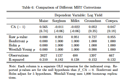
Use estadd to attach the raw and corrected p-values as scalars to each stored estimate, then export a single table. Instead of standard errors, the table shows the CA coefficient followed by a row for each p-value correction:

* attach corrected p-values to each stored estimate
    local crops     `" "Maize" "Sorghum" "Millet" "Groundnut" "Cowpea" "'
    local j = 1
    foreach c of local crops {
        estimates   restore `c'
        estadd      scalar raw_p   = `p`j''
        estadd      scalar bonf_p  = `p_bonf`j''
        estadd      scalar holm_p  = `p_holm`j''
        estadd      scalar wy_p    = `p_wy`j''
        estimates   drop `c'
        estimates   store `c'
        local       ++j
    }

* export summary table
    esttab          Maize Sorghum Millet Groundnut Cowpea ///
                        using "$answ/13-challenge.tex", replace ///
                        b(3) nostar ///
                        keep(CA) nodepvars ///
                        mtitles("Maize" "Sorghum" "Millet" ///
                            "Groundnut" "Cowpea") ///
                        stats(raw_p bonf_p holm_p wy_p N r2, ///
                            labels("Raw \textit{p}-value" ///
                                "Bonferroni \textit{p}" ///
                                "Holm \textit{p}" ///
                                "Westfall-Young \textit{p}" ///
                                "\midrule Observations" ///
                                "R-squared") ///
                            fmt(3 3 3 3 0 3)) ///
                        noobs booktabs nonum collabels(none) ///
                        nobaselevels nogaps fragment label ///
                        prehead("\begin{tabular}{l*{5}{c}} " ///
                            "\\[-1.8ex]\hline \hline \\[-1.8ex] " ///
                            "& \multicolumn{5}{c}{Dependent Variable: " ///
                            "Log Yield} \\ \midrule") ///
                        postfoot("\hline \hline \\[-1.8ex] " ///
                            "\multicolumn{6}{p{\linewidth}}{\small " ///
                            "\noindent \textit{Note}: Each column is a " ///
                            "separate OLS regression for the indicated " ///
                            "crop. Reported \textit{p}-values are for " ///
                            "the null hypothesis that " ///
                            "$\beta_{\text{CA}} = 0$. " ///
                            "Bonferroni and Holm adjust for 5 " ///
                            "hypotheses. Westfall-Young uses 1,000 " ///
                            "bootstrap replications.} " ///
                            "\end{tabular}")

Part 5 — Interpretation

Which crops have a statistically significant effect of CA at the 5% level using the raw p-value? Do any results lose significance under the corrections?
Why do the Westfall-Young adjusted p-values tend to be less conservative than the Bonferroni correction?

Assignment submission checklist

Solutions

Manual 2SLS 1, 2
Using ivreg2 1, 2, 3
Panel IV with xtivreg2 1, 2, 3
Instrument Diagnostics
Robust & Clustered Standard Errors 1, 2
Bootstrap Comparisons 1, 2
Wild Cluster Bootstrap
Randomization Inference 1, 2
Check That Your Code Runs
Challenge 13