Regression Discontinuity · Coding for Applied Economists

Learning Objectives

Following this assignment students should be able to:

Create and interpret binned-means RD plots

Estimate sharp (reduced-form) and fuzzy (IV) regression discontinuity designs

Use rdrobust for data-driven bandwidth selection and bias-corrected estimation

Assess bandwidth sensitivity of RD estimates

Run diagnostic checks: density tests and placebo outcome tests

Reading

Required Reading

We will cover Regression Discontinuity Designs (RDD).

Huntington-Klain, N. 2025. The Effect: An Introduction to Research Design and Causality, 2nd Edition. Chapter 20: Regression Discontinuity

Useful Stata Resources for RDD

Here are some helpful, accessible resources for learning how to implement Regression Discontinuity in Stata:

Video Tutorial: Regression Discontinuity Design in Stata (A practical walkthrough of basic RDD estimation and plotting).
UCLA IDRE Stata FAQ: How can I do a regression discontinuity analysis in Stata? (A clear step-by-step written guide).
World Bank DIME Wiki: Regression Discontinuity Design (Includes concept overview and Stata implementation tips).

Supplementary Reading

Garg, T. 2021. “Ecosystems and Human Health: The Local Benefits of Forest Cover in Indonesia.” Journal of Environmental Economics and Management, 54: 101365. The exercises this week use replication data from this paper, which studies how rural road construction in India affects agricultural burning and air pollution using a fuzzy RDD.

Lecture Notes

Exercises

RD Plot (10 pts)

For all the exercises this week we use data from the nationwide rural road construction program, Pradhan Mantri Gram Sadak Yojana (PMGSY) in India (Garg et al., 2024). In Garg et al. (2021), the authors examine how building rural roads causes movement of workers out of agriculture and induces farmers to use fire — a labor-saving but polluting technology — to clear agricultural residue or to make harvesting less labor-intensive. Under PMGSY, villages above a population threshold were eligible for a new all-weather road. The running variable v_pop measures each village’s population minus its state-specific threshold, so the cutoff is at zero.

Before doing any exercises, add a global to the top of this week’s assignment do-file that points to the rural roads data. Because the replication package is quite large, you will be accessing it from OneDrive. The start of your path will vary depending on your computer, but it will end with OneDrive - University of Arizona/Michler, Jeffrey David - (jdmichler)'s files - rural_roads.
```
* define rural roads data path (modify the start of the path for your computer)
	global			rr "C:/Users/YourName/OneDrive - University of Arizona/Michler, Jeffrey David - (jdmichler)'s files - rural_roads/data"
```
- Load "$rr/gjp_main_working.dta".
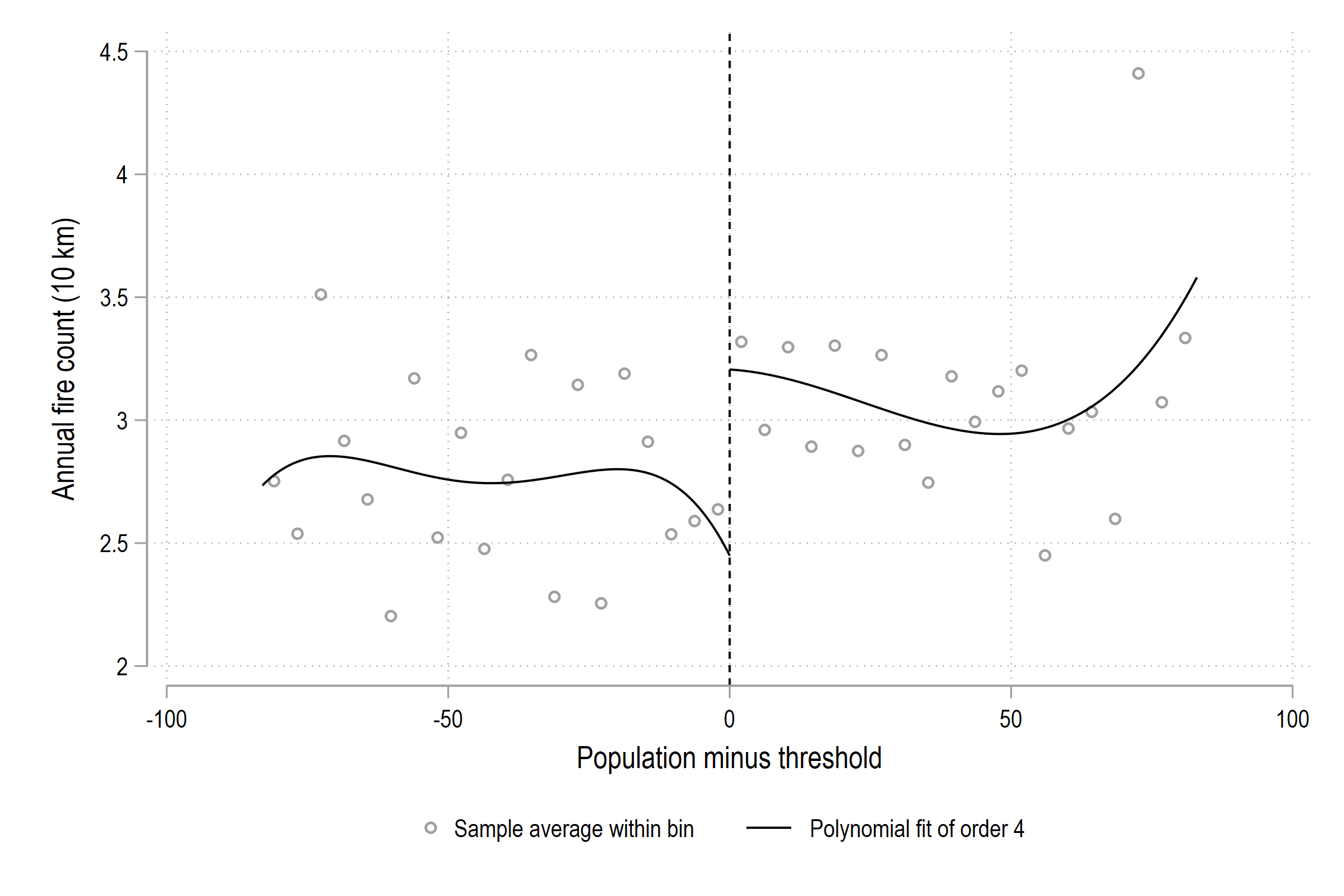
- Use rdplot to create a binned-means RD plot of fires10km (annual fire count within 10 km) against the running variable v_pop, with the cutoff at 0. Restrict the range to ±250 using the subset() or an if condition (if abs(v_pop) <= 250), set 20 bins per side with nbins(20 20), and add descriptive axis titles.
1. Export the graph and import it into your Overleaf document.
2. Is there visual evidence of a discontinuity in fire activity at the population threshold? Describe what you see.

Reduced-Form RD (15 pts)

In this exercise you will estimate a reduced-form (sharp) regression discontinuity using OLS. The Garg et al. (2021) data includes pre-computed linear terms for the RD polynomial: left captures the slope of the running variable below the cutoff and right captures the slope above the cutoff. The threshold indicator t equals 1 for villages above the population cutoff.

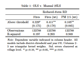
Run a reduced-form regression of fires10km on t left right, absorbing district-threshold (dist_thresh_id) and year (year) fixed effects using reghdfe, and clustering standard errors at the village_id level. Store as rf1.
Re-run the same regression but add triangular kernel weights [aw = kernel_tri_ik]. Store as rf2.
Run the kernel-weighted specification again but with pm25 as the outcome (add pm25_bl2001 as a baseline control). Store as rf3.

1. Export a three-column table to LaTeX:

* export reduced-form table
    esttab      rf1 rf2 rf3 using "$answ/14-rdd-ols.tex", replace ///
                    b(3) se(3) ///
                    keep(t) coeflabels(t "Above threshold") ///
                    star(* 0.10 ** 0.05 *** 0.01) ///
                    mtitles("Fires" "Fires (wt)" "PM 2.5 (wt)") ///
                    stats(N r2, labels("Observations" "R-squared") ///
                        fmt(0 3)) ///
                    noobs booktabs nonum collabels(none) ///
                    nobaselevels nogaps fragment label ///
                    prehead("\begin{tabular}{l*{3}{c}} " ///
                        "\\[-1.8ex]\hline \hline \\[-1.8ex] " ///
                        "& \multicolumn{3}{c}{Reduced-Form RD}" ///
                        " \\ \midrule") ///
                    postfoot("\hline \hline \\[-1.8ex] " ///
                        "\multicolumn{4}{p{\linewidth}}{\small " ///
                        "\noindent \textit{Note}: Dependent " ///
                        "variable indicated in column header. " ///
                        "All models include district-threshold " ///
                        "and year FE. Columns 2--3 use " ///
                        "triangular kernel weights. Std.\ errors " ///
                        "clustered at village level. " ///
                        "* p$<$0.10, ** p$<$0.05, " ///
                        "*** p$<$0.01.} " ///
                        "\end{tabular}")

2. Interpret the coefficient on t (the threshold) in the unweighted fires regression. What does it mean substantively?

3. How does adding kernel weights change the estimate? Why might this happen?

Using `rdrobust` (15 pts)

In this exercise you will use the rdrobust package for data-driven bandwidth selection and then check how sensitive the estimate is to bandwidth choice — the RDD equivalent of the specification charts from Week 10.

Run rdrobust fires10km v_pop, c(0) and note the conventional estimate, the bias-corrected estimate, and the optimal bandwidth selected.

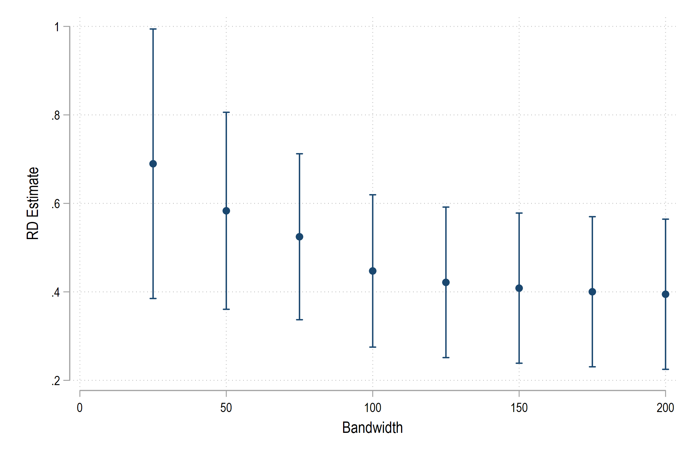
1. What bandwidth does rdrobust select by default? How many observations fall within that bandwidth?

Now check bandwidth sensitivity. Loop over a set of bandwidths (25, 50, 75, 100, 150, 200) and store the conventional estimate and confidence interval at each bandwidth. Use the code below as a template:

* bandwidth sensitivity
	matrix			bw_results = J(6, 4, .)
	local			bandwidths 25 50 75 100 150 200
	local			row = 1

	foreach bw of local bandwidths {
		rdrobust	fires10km v_pop, c(0) h(`bw')
		matrix		bw_results[`row', 1] = `bw'
		matrix		bw_results[`row', 2] = e(tau_cl)
		matrix		bw_results[`row', 3] = e(ci_l_cl)
		matrix		bw_results[`row', 4] = e(ci_r_cl)
		local		++row
	}

Convert the matrix to a dataset and create a coefplot-style graph showing the point estimate ± 95% CI at each bandwidth. Add a horizontal reference line at zero.

* convert matrix to dataset for plotting
	preserve
	clear
	svmat           bw_results
	rename         (bw_results1 bw_results2 bw_results3 ///
	                   bw_results4) (bandwidth estimate ///
                       ci_lo ci_hi)

	twoway         (rcap ci_lo ci_hi bandwidth, lcolor(navy)) ///
                       (scatter estimate bandwidth, ///
                       mcolor(navy) msymbol(circle)), ///
                       yline(0, lcolor(maroon) lpattern(dash)) ///
                       ytitle("RD Estimate") ///
                       xtitle("Bandwidth") ///
                       legend(off) ///
                       graphregion(color(white))
	graph export	"$answ/14-rdd-bw.png", replace
	restore

2. Export the figure and import it into your Overleaf document.

3. Is the fire-count estimate stable as you widen the bandwidth, or does it change substantially?

First Stage (10 pts)

The Garg et al. (2021) RDD is fuzzy: crossing the population threshold increases the probability of receiving a road but does not guarantee it. Before running the fuzzy RD, we need to verify that the first stage is strong — that the threshold indicator actually predicts road construction.
- Define a global for the baseline controls:
```
* baseline controls
    global      blcontrols primary_school med_center elect ///
                    tdist irr_share ln_land pc01_lit_share ///
                    pc01_sc_share bpl_landed_share ///
                    bpl_inc_source_sub_share bpl_inc_250plus
```
- Run the first-stage regression: regress receivedroad on t left right $blcontrols using reghdfe, with triangular kernel weights [aw = kernel_tri_ik], absorbing year and dist_thresh_id fixed effects, and clustering standard errors at village_id. Store as fs.
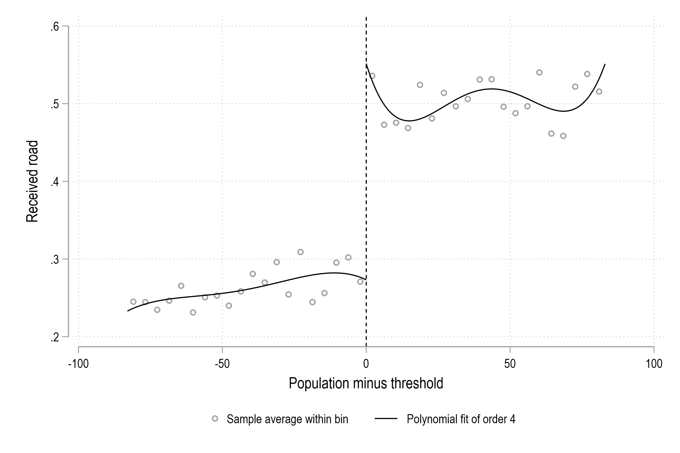
1. Use rdplot to visualize the first stage. Plot receivedroad against v_pop with the cutoff at 0. Restrict to abs(v_pop) <= 250 and use 20 bins per side. Export the figure and import it into your Overleaf document.

2. What is the coefficient on t? Interpret it in words: by how many percentage points does crossing the threshold increase the probability of receiving a road?

3. Is the first stage strong? Check the F-statistic against the conventional rule-of-thumb threshold of $F > 10$.

Fuzzy RDD (15 pts)

Now we estimate the fuzzy RD — the causal effect of actually receiving a road on fire activity and air pollution. Following the IV logic from Week 13, we use the population threshold t as an instrument for receivedroad.

Run the fuzzy RD for fires (fires10km) using ivreghdfe and instrumenting for receivedroad with t.
Include as exogenous left-hand-side variables left right and the baseline controls.
Absorb district-threshold (dist_thresh_id) and year (year) fixed effects, and clustering standard errors at the village_id level.
Use triangular kernel weights [aw = kernel_tri_ik].
Store results as iv_fires.
Finally, calculate the control group mean for fires within the effective sample (if e(sample) & t == 0) and store it as a scalar called depvarmean.
Run the same specification for pm25 (replace fires10km with pm25 and fires2001_10km with pm25_bl2001 as the baseline control). Store as iv_pm. and again calculate the control group mean for pm25 within the effective sample and store it as depvarmean.

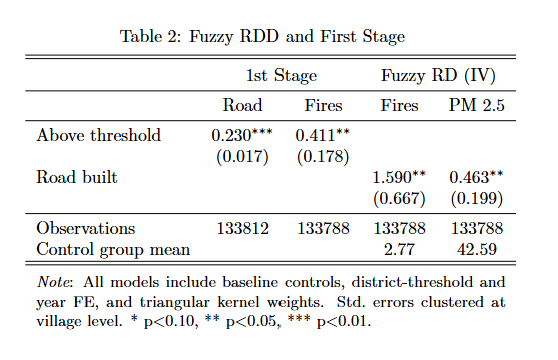
1. Export a four-column table. Make sure you still have the reduced-form estimates from Exercise 2 (rf2) and the first-stage estimate from Exercise 4 (fs) stored.

* four-column table
    esttab      fs rf2 iv_fires iv_pm ///
                    using "$answ/14-rdd-fuzzy.tex", replace ///
                    b(3) se(3) ///
                    keep(t receivedroad) ///
                    coeflabels(t "Above threshold" ///
                        receivedroad "Road built") ///
                    star(* 0.10 ** 0.05 *** 0.01) ///
                    mtitles("Road" "Fires" "Fires" "PM 2.5") ///
                    stats(N depvarmean, ///
                        labels("Observations" ///
                            "Control group mean") ///
                        fmt(0 2)) ///
                    noobs booktabs nonum collabels(none) ///
                    nobaselevels nogaps fragment label ///
                    prehead("\begin{tabular}{l*{4}{c}} " ///
                        "\\[-1.8ex]\hline \hline \\[-1.8ex] " ///
                        "& \multicolumn{2}{c}{1st Stage} " ///
                        "& \multicolumn{2}{c}{Fuzzy RD (IV)}" ///
                        " \\ \midrule") ///
                    postfoot("\hline \hline \\[-1.8ex] " ///
                        "\multicolumn{5}{p{\linewidth}}{\small " ///
                        "\noindent \textit{Note}: All models " ///
                        "include baseline controls, " ///
                        "district-threshold and year FE, and " ///
                        "triangular kernel weights. Std.\ errors " ///
                        "clustered at village level. " ///
                        "* p$<$0.10, ** p$<$0.05, " ///
                        "*** p$<$0.01.} " ///
                        "\end{tabular}")

2. Does road construction increase or decrease air pollution? Is this consistent with the direction of the fire effect?

Density Test (10 pts)

If villages can manipulate their population to cross the eligibility threshold, the quasi-random assignment at the cutoff breaks down. We test for manipulation by checking whether the density of the running variable is smooth at the cutoff.
- Load "$rr/pmgsy_runningvar.dta" (this file contains the running variable for the full universe of villages, not just the analysis sample).
- Keep observations within ±500 of the threshold (abs(v_pop) <= 500).
- Run the McCrary density test using the dc_density command (make sure you’ve downloaded it from the course website and copied the dc_density program into your ado directory):
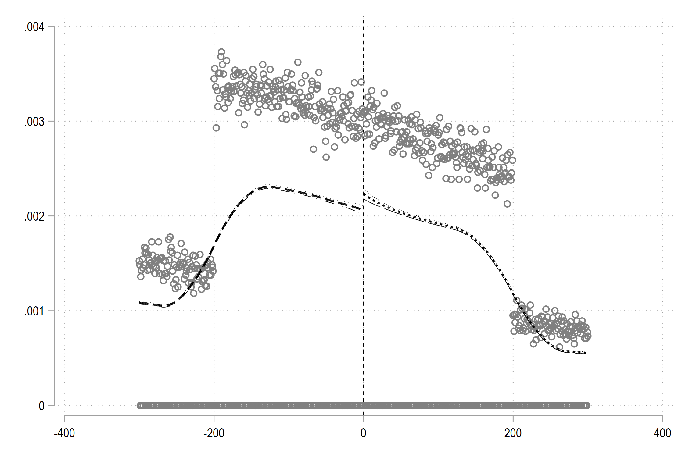
(Note: this will automatically run the test and export the graph. If you have an earlier dc_density graph, you may get a “already exists” error on the generated variables; you can type cap drop Xj Yj r0 fhat se_fhat before running it).
```
* run density test
    dc_density      v_pop, breakpoint(0) ///
                        generate(Xj Yj r0 fhat se_fhat) ///
                        graphname("$answ/14-rdd-density-1.png")
```
1. Export the graph and import it into your Overleaf document.
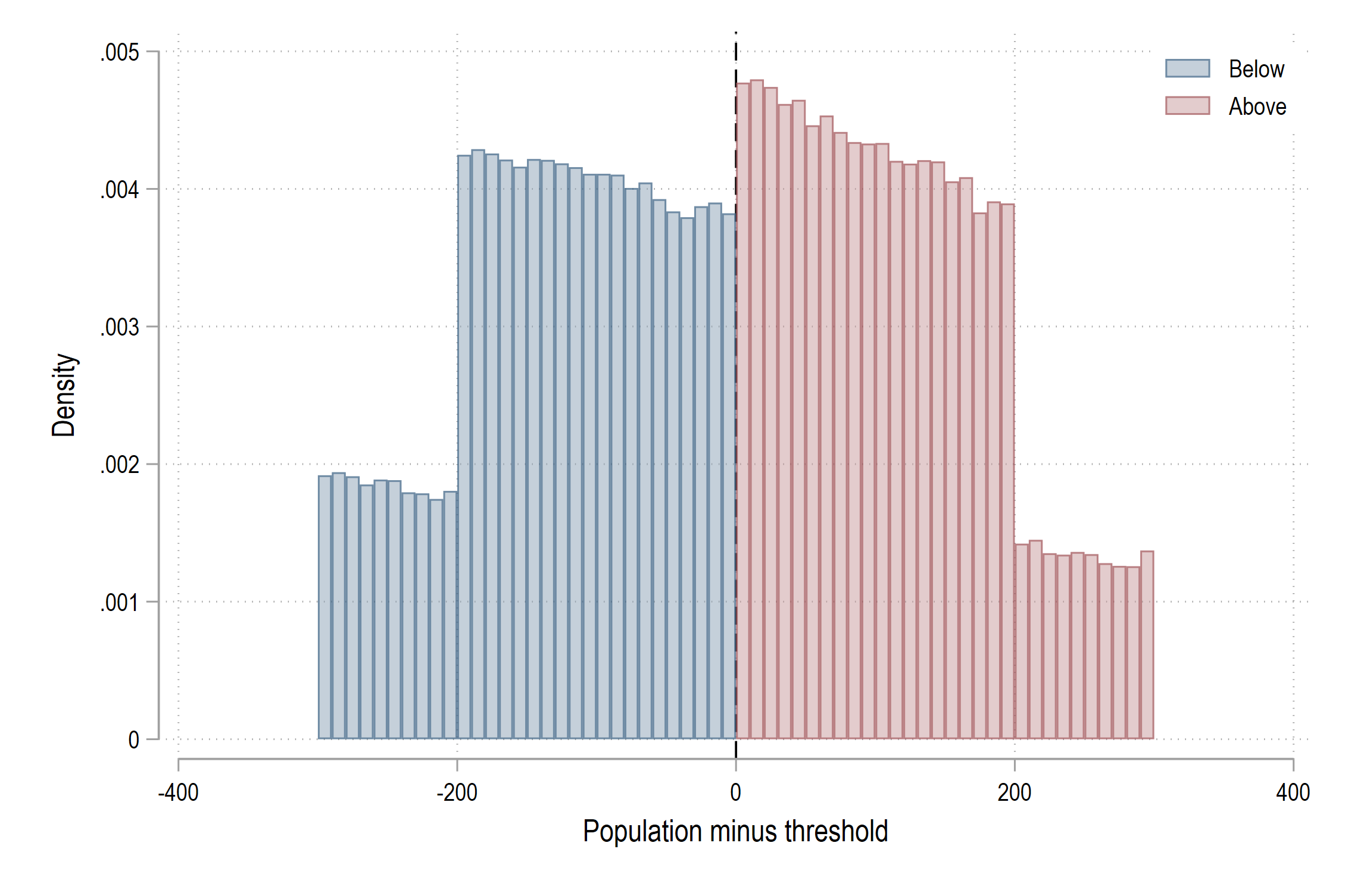
- Next, to match the formatting of our other graphs, create a standard histogram of the running variable with a vertical line at the cutoff:
```
* custom histogram of running variable
	twoway         (histogram v_pop if v_pop < 0, ///
                        width(10) color(navy%50)) ///
                        (histogram v_pop if v_pop >= 0, ///
                        width(10) color(maroon%50)), ///
                        xline(0, lcolor(black) lpattern(dash)) ///
                        xtitle("Population minus threshold") ///
                        ytitle("Density") ///
                        legend(order(1 "Below" 2 "Above") ///
                            ring(0) pos(1)) ///
                        graphregion(color(white))
	graph export	"$answ/14-rdd-density-2.png", replace
```
2. Export the histogram and import it into your Overleaf document.

3. What is the estimated log-difference in height at the cutoff (the parameter theta in the McCrary test output) and its standard error? Is there evidence of manipulation?

Placebo Outcomes (15 pts)

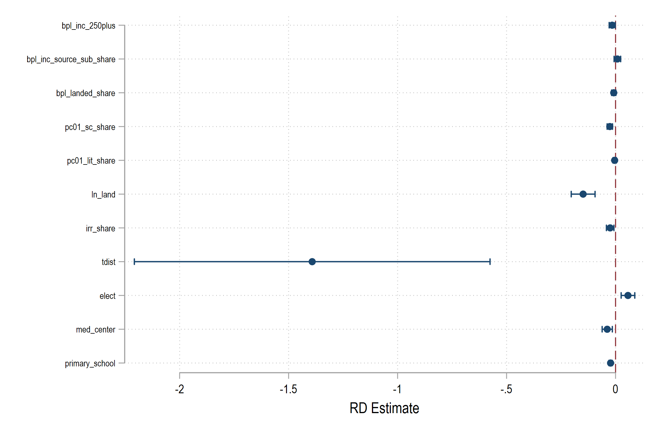
If the RDD is valid, baseline covariates — things determined before treatment — should not jump at the cutoff. This is the RDD analogue of the balance checks you would run in an experiment or the pre-trend tests in DiD (Week 12).

Load "$rr/gjp_main_working.dta".
Define the list of baseline covariates to test:

* placebo outcome list
	local           placebos primary_school med_center elect ///
                        tdist irr_share ln_land pc01_lit_share ///
                        pc01_sc_share bpl_landed_share ///
                        bpl_inc_source_sub_share bpl_inc_250plus

Loop over each variable in the list and run rdrobust with that variable as the outcome and v_pop as the running variable (cutoff at 0). Store estimates in a matrix for plotting:

* run placebo tests
    local           nvars : word count `placebos'
    matrix          placebo_res = J(`nvars', 3, .)
    matrix rownames placebo_res = `placebos'
    local           row = 1

    foreach var of local placebos {
        qui rdrobust        `var' v_pop, c(0)
        matrix              placebo_res[`row', 1] = e(tau_cl)
        matrix              placebo_res[`row', 2] = e(ci_l_cl)
        matrix              placebo_res[`row', 3] = e(ci_r_cl)
        local               ++row
    }

Convert the matrix to a dataset and create a coefficient plot of all placebo estimates with 95% CIs and a vertical reference line at zero.

* convert to dataset for plotting
    preserve
    clear
    svmat           placebo_res
    rename          (placebo_res1 placebo_res2 placebo_res3) ///
                        (estimate ci_lo ci_hi)
    gen             id = _n
    local           row = 1
    foreach var of local placebos {
        label define    idlbl `row' "`var'", add
        local           ++row
    }
    label values    id idlbl

    twoway          (rcap ci_lo ci_hi id, horizontal ///
                        lcolor(navy)) ///
                        (scatter id estimate, ///
                        mcolor(navy) msymbol(circle)), ///
                        xline(0, lcolor(maroon) lpattern(dash)) ///
                        xtitle("RD Estimate") ///
                        ytitle("") ///
                        ylabel(1/`nvars', valuelabel angle(0) ///
                            labsize(vsmall)) ///
                        legend(off) ///
                        graphregion(color(white))
    graph export    "$answ/14-rdd-placebo.png", replace
    restore

1. Export the graph and import into your Overleaf document.

2. Do any baseline covariates show a statistically significant discontinuity at the 5% level?

3. If one out of eleven variables is significant at the 10% level, is that a concern? Why or why not? (Hint: think about what you would expect by random chance when running multiple tests.)

Check That Your Code Runs (10 pts)

Sometimes you think you’re code runs, but it only actually works because of something else you did previously. To make sure it actually runs you should save your work and then run it in a clean environment.

Follow these steps in to make sure your code really runs:
1. Restart Stata by closing the instance of Stata that you have open.
2. When you reopen Stata, type in the command line clear all. Or, better yet, put clear all at the top of your .do file, after the preamble but before any commands.
3. Rerun your entire homework assignment by clicking the Execute button to make sure it runs from start to finish and produces the expected results.
4. Make sure that you saved your code with the name of the assignment number (i.e., assignment_01). You should see the file in your git repo on your machine.
5. Make sure that your code will run on other computers (relevant for all assignments after the first assignment)
  - No cd. Use a project.do file instead to set directories
  - Use only relative paths in files other than the project.do file
  - Use / not \ for paths

Challenge 14 (Challenge - 20 pts)

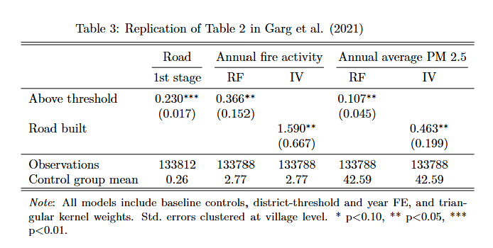
This challenge ties together the full RDD workflow from the week: first stage, reduced form, fuzzy RD, bandwidth sensitivity, and subgroup analysis. You will replicate parts of the main results from Garg et al. (2021) and present them in publication-quality tables and figures.

Part 1 — Replicate Table 2

Replicate the core results of Table 2 from Garg et al. (2021). The table has five columns: (1) first stage, (2) reduced-form fires, (3) IV fires, (4) reduced-form PM 2.5, and (5) IV PM 2.5.

Load "$rr/gjp_main_working.dta".
Define the baseline controls (same as previous exercises).
Run the following five specifications using either reghdfe or ivreghdfe as appropriate, all with triangular kernel weights, district-threshold and year FE, and standard errors clustered at the village level:
1. First stage: regress receivedroad on t, left, right, and $blcontrols. Store as fs.
2. Reduced-form fires: regress fires10km on t, left, right, fires2001_10km, and $blcontrols. Store as rf_fires.
3. IV fires: regress fires10km on left, right, fires2001_10km, and $blcontrols, treating receivedroad as endogenous and t as the instrument. Store as iv_fires.
4. Reduced-form PM 2.5: Same as (2) but with pm25 and baseline pm25_bl2001. Store as rf_pm.
5. IV PM 2.5: Same as (3) but with pm25 and baseline pm25_bl2001. Store as iv_pm.
For each model, use estadd scalar depvarmean = r(mean) to attach the control-group mean for villages where t == 0.
Export all five columns to a single LaTeX table:

* export table 2 replication
    esttab          fs rf_fires iv_fires rf_pm iv_pm ///
                        using "$answ/14-challenge-tab2.tex", replace ///
                        b(3) se(3) ///
                        keep(t receivedroad) ///
                        coeflabels(t "Above threshold" ///
                            receivedroad "Road built") ///
                        star(* 0.10 ** 0.05 *** 0.01) ///
                        mgroups("Road" "Annual fire activity" ///
                            "Annual average PM 2.5", ///
                            pattern(1 1 0 1 0) ///
                            prefix(\multicolumn{@span}{c}{) ///
                            suffix(}) span ///
                            erepeat(\cmidrule(lr){@span})) ///
                        mtitles("1st stage" "RF" "IV" "RF" "IV") ///
                        stats(N depvarmean, ///
                            labels("Observations" ///
                                "Control group mean") ///
                            fmt(0 2)) ///
                        noobs booktabs nonum collabels(none) ///
                        nobaselevels nogaps fragment label ///
                        prehead("\begin{tabular}{l*{5}{c}} " ///
                            "\\[-1.8ex]\hline \hline \\[-1.8ex]") ///
                        postfoot("\hline \hline \\[-1.8ex] " ///
                            "\multicolumn{6}{p{\linewidth}}{\small " ///
                            "\noindent \textit{Note}: All models " ///
                            "include baseline controls, " ///
                            "district-threshold and year FE, and " ///
                            "triangular kernel weights. Std.\ errors " ///
                            "clustered at village level. " ///
                            "* p$<$0.10, ** p$<$0.05, " ///
                            "*** p$<$0.01.} " ///
                            "\end{tabular}")

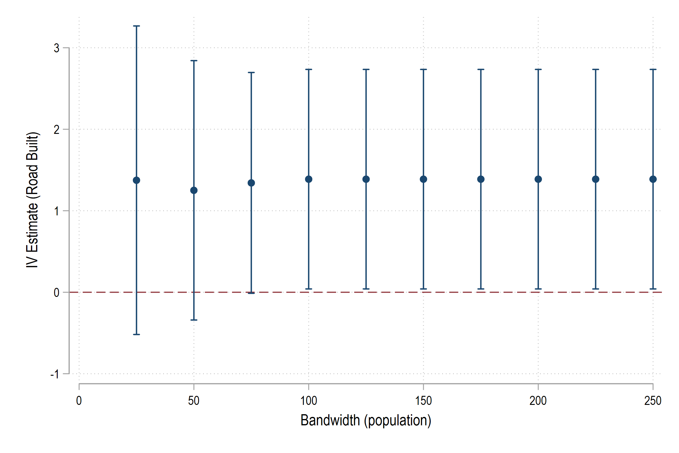
Part 2 — Bandwidth Sensitivity

Using the IV fires specification from Part 1, re-estimate the model at several bandwidth windows. You can impose different bandwidths by restricting the sample to abs(v_pop) <= bw. Loop over bandwidths of 25, 50, 75, 100, 150, 200, and 250.

* bandwidth sensitivity for IV fires
    matrix          bw_iv = J(10, 4, .)
    local           bws 25 50 75 100 125 150 175 200 225 250
    local           row = 1

    foreach bw of local bws {
        cap noisily ivreghdfe fires10km (receivedroad = t) ///
                        left right fires2001_10km $blcontrols ///
                        if abs(v_pop) <= `bw', ///
                        a(year dist_thresh_id) cluster(village_id)
        if _rc == 0 {
            matrix	bw_iv[`row', 1] = `bw'
            matrix	bw_iv[`row', 2] = _b[receivedroad]
            matrix	bw_iv[`row', 3] = _b[receivedroad] - ///
                        1.96 * _se[receivedroad]
            matrix	bw_iv[`row', 4] = _b[receivedroad] + ///
                        1.96 * _se[receivedroad]
        }
        local		++row
    }

Convert the matrix to a dataset and create a coefficient plot showing the IV estimate ± 95% CI at each bandwidth. Add a horizontal reference line at zero. Export and import into Overleaf.

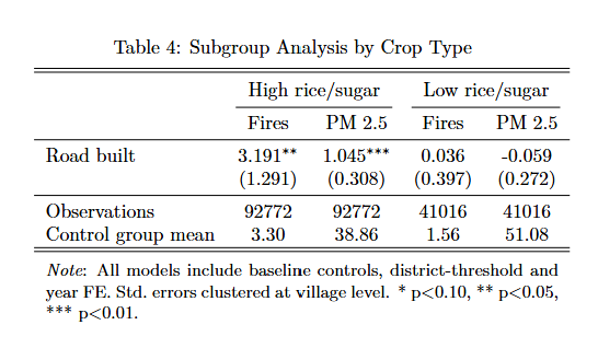
Part 3 — Subgroup Analysis

The paper argues that road access increases agricultural fires because roads reduce the cost of transporting crops to market, making mechanized harvesting (which leaves flammable stubble) more profitable. This mechanism should be strongest in areas that grow crops whose residue is commonly burned (rice and sugarcane).

Using the main working data, create indicators for “high rice or high sugar” districts — the variables rice_hi and sugar_hi are already defined in the dataset (created during the merge step). Generate a combined indicator:

* subgroup indicators
    gen          burning_crops = (rice_hi == 1 | sugar_hi == 1)

Re-run the IV fires and IV PM 2.5 specifications separately for burning_crops == 1 and burning_crops == 0. Store as iv_fires_hi, iv_pm_hi, iv_fires_lo, iv_pm_lo. Save the control-group mean for each.
Export a four-column table to LaTeX:

* subgroup table
    esttab      iv_fires_hi iv_pm_hi iv_fires_lo iv_pm_lo ///
                  using "$answ/14-challenge-subgroup.tex", ///
                  replace ///
                  b(3) se(3) ///
                  keep(receivedroad) ///
                  coeflabels(receivedroad "Road built") ///
                  star(* 0.10 ** 0.05 *** 0.01) ///
                  mgroups("High rice/sugar" ///
                        "Low rice/sugar", ///
                        pattern(1 0 1 0) ///
                        prefix(\multicolumn{@span}{c}{) ///
                        suffix(}) span ///
                        erepeat(\cmidrule(lr){@span})) ///
                  mtitles("Fires" "PM 2.5" ///
                        "Fires" "PM 2.5") ///
                  stats(N depvarmean, ///
                        labels("Observations" ///
                            "Control group mean") ///
                        fmt(0 2)) ///
                  noobs booktabs nonum collabels(none) ///
                  nobaselevels nogaps fragment label ///
                  prehead("\begin{tabular}{l*{4}{c}} " ///
                        "\\[-1.8ex]\hline \hline \\[-1.8ex]") ///
                  postfoot("\hline \hline \\[-1.8ex] " ///
                        "\multicolumn{5}{p{\linewidth}}{\small " ///
                        "\noindent \textit{Note}: All models " ///
                        "include baseline controls, " ///
                        "district-threshold and year FE. " ///
                        "Std.\ errors clustered at village " ///
                        "level. " ///
                        "* p$<$0.10, ** p$<$0.05, " ///
                        "*** p$<$0.01.} " ///
                        "\end{tabular}")

Part 4 — Interpretation

Does the effect of road construction on fires concentrate in high rice/sugar regions? What does that tell you about the mechanism linking roads to fires?
Why is the subgroup analysis informative for the paper’s argument, and how does it differ from simply adding an interaction term?

Assignment submission checklist

Solutions

RD Plot 1, 2
Reduced-Form RD 1, 2
Using rdrobust 1, 2
First Stage 1, 2
Fuzzy RDD 1, 2
Density Test 1, 2, 3
Placebo Outcomes 1, 2
Check That Your Code Runs
Challenge 14 1, 2, 3, 4