Learning Objectives
Following this assignment students should be able to:
- Create reproducible train/test splits and understand why holdout evaluation matters
- Use
lasso linearandelasticnet linearfor penalized regression and variable selection- Fit random forest and gradient boosting models using H2O’s
h2omlcommands- Compare multiple models on out-of-sample prediction accuracy (MSE)
- Interpret ML models using variable importance, partial dependence plots, and SHAP values
- Distinguish between prediction and causal inference in applied economics
Reading
Topics
- H20 integration
- Lasso
- Random forest
- Gradient boosting
Readings
- Video (4 min): How to set up H2O in Stata
- Video (7 min): Lasso for prediction and model selection
- Video (3 min): Random forest and gradient boosting
Lecture Notes
Exercises
-
Setup and Train/Test Split (15 pts)
Before fitting any ML models, we need to prepare our data and create a proper train/test split. For all exercises this week we use
plot_dataset.dta— a plot-crop level dataset on agricultural production from Ethiopia, Malawi, Mali, Niger, Nigeria, Tanzania, and Uganda across 8 waves. The unique identifier isplot_id_obs season. You can download the data from the list of datasets page.The prediction task for this week is to forecast crop yield (
yield_kg) using crop type, plot characteristics, input use, manager demographics, soil quality, geography, and shock variables.- Load
plot_dataset.dta.
1. Examine the data. How many observations are there? What is the mean yield?
- Create a random train/test split using
splitsample. Split 70% training and 30% test, generate a variable calledsample, and set the random seed to8675309. Label the values ofsampleso that 1 is “Training” and 2 is “Testing”.
2. How many observations are in the training set? How many are in the test set? Report the numbers.
- Load
-
Lasso for Prediction (15 pts)
Use Stata’s native
lasso linearcommand to predict crop yield using a large set of covariates fromplot_dataset.dta. The lasso will automatically select which variables to keep by shrinking unimportant coefficients to zero.- Create a global macro called
inputsthat includes the following variables:seed_kg,nitrogen_kg,total_labor_days,total_hired_labor_days,improved,used_pesticides,organic_fertilizer,irrigated,intercropped,age_manager,female_manager,formal_education_manager,plot_slope,elevation,dist_market,dist_popcenter,soil_fertility_index,crop_shock,drought_shock, and factor variablesi.crop,1.agro_ecological_zone,i.waveandi.country. - Using the training set only (
if sample == 1), runlasso linearto predictyield_kgusing the global macro$inputs. - Store the estimates from this model (e.g.,
estimates store cv). - Run a second model on the same training set using adaptive lasso by adding the
selection(adaptive)option to the previous command. - Store the estimates from the adaptive lasso model (e.g.,
estimates store adpt).
1. Compare the selected variables using
lassocoeffor both stored models. Which coefficients are in the standard lasso but not in the adaptive lasso? Which ones are in the adaptive lasso but not in the standard lasso?2. Create cross-validation plots for both models using
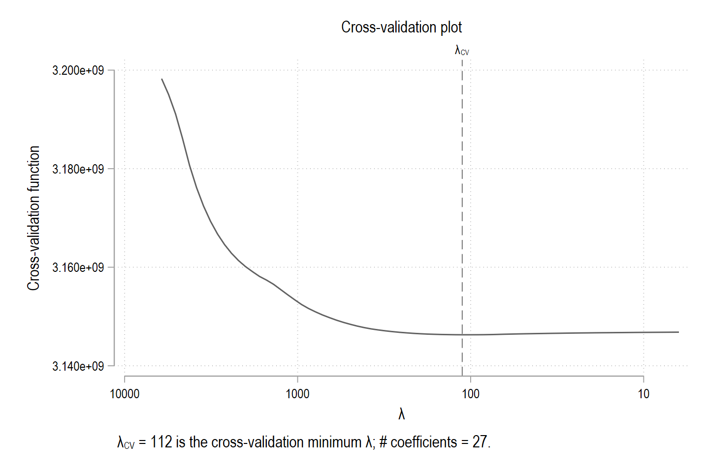
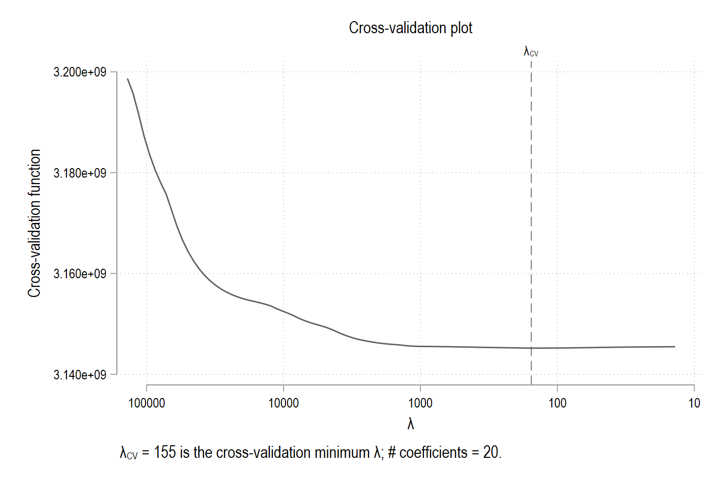
cvplot(remember to useestimates restorebefore plotting each one). Export the graphs to Overleaf.- Compare the in-sample and out-of-sample MSE for both models using
lassogofwith theover(sample)andpostselectionoptions.
3. Which model does best at out-of-sample prediction?
- For the final model comparison challenge at the end of the assignment, you will need the out-of-sample predictions from the standard lasso model. Use
estimates restore cvto make it the active model, then usepredict yhat_lassoto generate predictions for the entire dataset.
- Create a global macro called
-
Elastic Net and Ridge (15 pts)
Lasso (α = 1) sets some coefficients to exactly zero. Ridge (α = 0) shrinks all coefficients but keeps every variable. Elastic net blends both. In this exercise, compare all three using
plot_dataset.dta.- Using the training set and the global macro
$inputs, runelasticnet linearwithalpha(1)(this is lasso — confirm it matches Exercise 2). Save results asalph1. - Run elastic net with
alpha(0.5). Save results asalph5. - Run ridge with
alpha(0). Save results asalph0. - Compare results using
lassocoef.
If a model does not converge, remember you can change the search space and/or the stopping rule.
-
How many variables with nonzero coefficients are in each model?
-
How does the number of selected variables change as α moves from 1 (lasso) to 0.5 (elastic net) to 0 (ridge)? Why?
-
Compare the out-of-sample MSE across the three models. Which performs best? Is the difference large?
- For the final model comparison challenge, you will need the predictions from your best-performing elastic net model. Assume
alpha(0.5)is the best. Useestimates restore alph5and then usepredict yhat_enetto generate predictions for the entire dataset.
- Using the training set and the global macro
-
Random Forest (15 pts)
Random forest builds many decision trees on random subsets of data and variables, then averages their predictions. This exercise uses H2O’s
h2oml rfregresscommand withplot_dataset.dta. Make sure H2O is initialized and your data is loaded in an H2O frame (from Exercise 1). If you have restarted Stata, re-runh2o initand push the training and testing sets to H2O using_h2oframe put.- Initialize the H2O cluster with
h2o init. If you have not installed Java, follow the instructions on the Computer Setup page first. - Push the training data to an H2O frame named
train_frameand make it current. Then push the testing data to an H2O frame namedtest_frame. - Fit a random forest to predict
yield_kgon the training set using the same set of predictors as in previous exercises. Use 200 trees, a maximum depth of 10, and 5-fold cross-validation:
Note: When using
h2oml, do not include thei.prefix for factor variables. H2O handles categorical variables internally. Passwaveandadmin_1withouti.. So instead of using the global macro use the following local macro:local h2o_inputs = subinstr("$inputs", "i.", "", .)- Set the testing frame and compute the out-of-sample MSE using
h2omlgof:
-
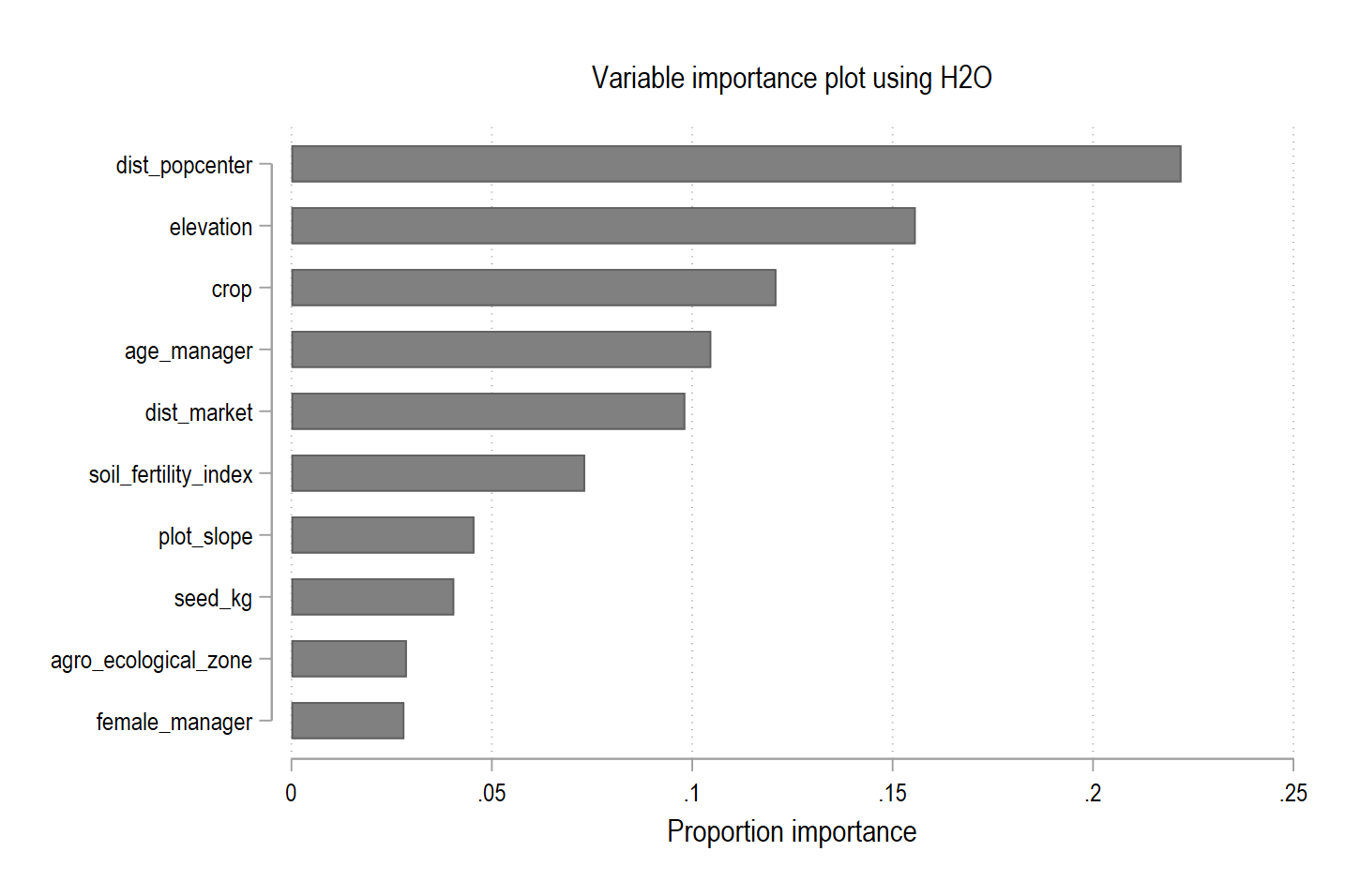
Generate a variable importance plot, export it, and import it into Overleaf.
-
What is the out-of-sample MSE? How does it compare to the lasso MSE from Exercise 2?
-
Which three variables are most important according to the variable importance plot? Does this match your economic intuition about what drives crop yield?
- For the final model comparison challenge, you will need the predictions from your random forest model. Use
predict yhat_rfto generate predictions for the entire dataset before moving on.
- Initialize the H2O cluster with
-
Gradient Boosting (15 pts)
Gradient boosting builds trees sequentially — each new tree corrects the errors of the ensemble. This exercise uses H2O’s
h2oml gbregresscommand withplot_dataset.dta.- Fit a gradient boosting model to predict
yield_kgon the training set using the local macro we created in the previous exercise. Use 500 trees, a maximum depth of 5, a learning rate of 0.05, and 5-fold cross-validation:
1. What is the out-of-sample MSE on the testing frame using
h2omlgof?- For the final model comparison challenge, you will need the predictions from your optimal gradient boosting model. Use
predict yhat_gbmto generate predictions for the entire dataset before estimating any further models.
2. Re-run the model with a higher learning rate:
lrate(0.3). What happens to the out-of-sample MSE? Why does a smaller learning rate often produce better predictions, even though it requires more trees?
- Fit a gradient boosting model to predict
-
SHAP and Variable Importance (15 pts)
ML models are powerful predictors but can be hard to interpret. This exercise uses H2O’s interpretation tools to understand why the gradient boosting model makes the predictions it does using
plot_dataset.dta. Make sure your GBM model from the previous exercise is the most recently estimated H2O model (theh2omlgraphcommands operate on the lasth2omlmodel). If needed, re-estimate the GBM model.-
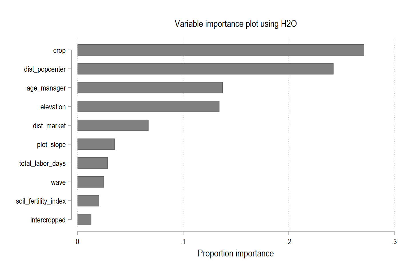
Generate a variable importance plot, export it, and import it into Overleaf.
-
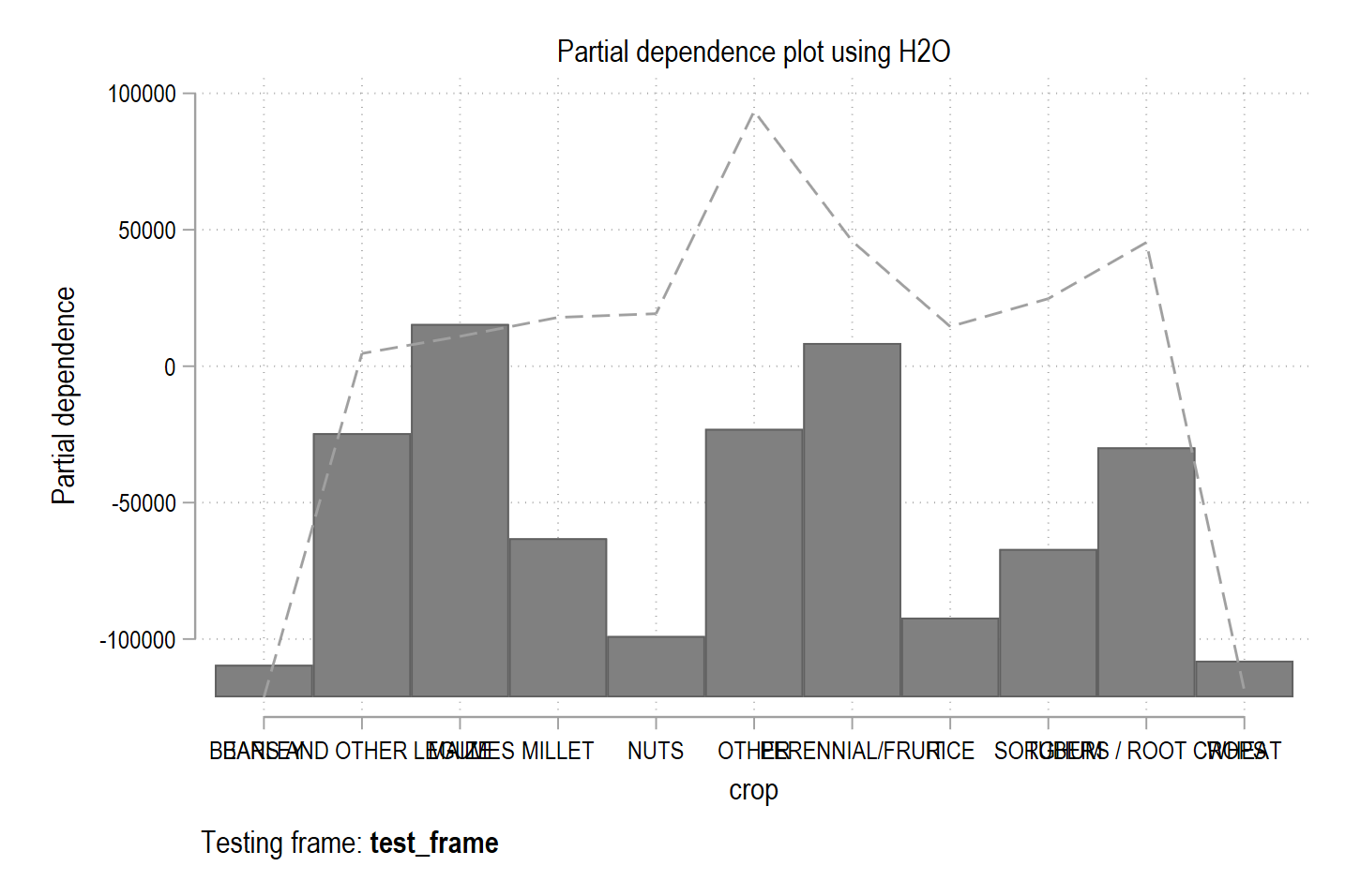
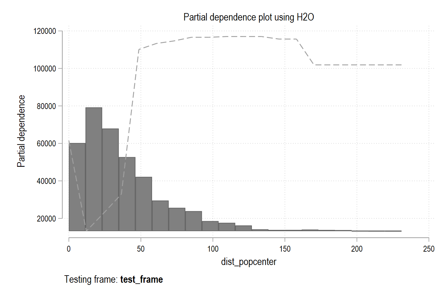
Generate partial dependence plots for the two most important predictors identified by the variable importance plot. Export them and import them into Overleaf.
-
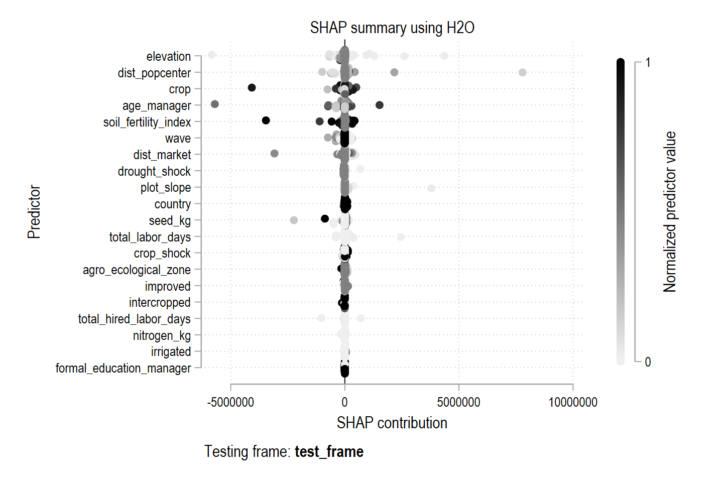
Generate a SHAP summary plot, export it, and import it into Overleaf.
-
Examine the SHAP summary plot. For the top three variables, describe the relationship between the variable’s value (shading) and its SHAP value (horizontal position). For example: “Higher nitrogen application (darker dots) is associated with positive SHAP values, meaning it pushes yield predictions upward.”
-
-
Check That Your Code Runs (10 pts)
Sometimes you think you’re code runs, but it only actually works because of something else you did previously. To make sure it actually runs you should save your work and then run it in a clean environment.
Follow these steps in to make sure your code really runs:
-
Restart Stata by closing the instance of Stata that you have open.
-
When you reopen Stata, type in the command line
clear all. Or, better yet, putclear allat the top of your.dofile, after the preamble but before any commands. -
Rerun your entire homework assignment by clicking the
Executebutton to make sure it runs from start to finish and produces the expected results. -
Make sure that you saved your code with the name of the assignment number (i.e.,
assignment_01). You should see the file in your git repo on your machine. -
Make sure that your code will run on other computers (relevant for all assignments after the first assignment)
- No
cd. Use aproject.dofile instead to set directories - Use only relative paths in files other than the
project.dofile - Use
/not\for paths
- No
-
-
Challenge 15 (Challenge - 20 pts)
Part 1 — Model Comparison
Now that you have fit lasso, elastic net, random forest, and gradient boosting on
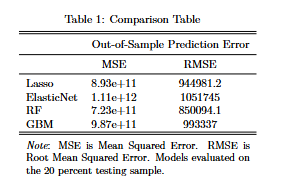
plot_dataset.dta, it is time to compare them. Which algorithm is best suited for this specific data generating process?- Create a matrix to collect the results and loop over the models to compute MSE and RMSE:
* collect results
    matrix          compare = J(4, 2, .)
    matrix rownames compare = Lasso ElasticNet RF GBM
    matrix colnames compare = MSE RMSE

    local           row = 1
    foreach model in lasso enet rf gbm {
        gen         sq_err_`model' = (yield_kg - yhat_`model')^2
        sum         sq_err_`model' if sample == 2
        matrix      compare[`row', 1] = r(mean)
        matrix      compare[`row', 2] = sqrt(r(mean))
        local       ++row
    }
    matrix list     compare, format(%12.1f)
1. Export a LaTeX table of the results for your Overleaf document:
* export results to latex
    esttab      matrix(compare) using "$answ/15-ml-compare.tex", replace ///
                    nomtitles noobs booktabs ///
                    collabels("MSE" "RMSE") ///
                    fragment label ///
                    prehead("\begin{tabular}{l*{2}{c}} " ///
                        "\\[-1.8ex]\hline \hline \\[-1.8ex] " ///
                        "& \multicolumn{2}{c}{Out-of-Sample Prediction Error} " ///
                        "\\ \midrule") ///
                    postfoot("\hline \hline \\[-1.8ex] " ///
                        "\multicolumn{3}{p{\linewidth}}{\small " ///
                        "\noindent \textit{Note}: MSE is Mean Squared Error. " ///
                        "RMSE is Root Mean Squared Error. Models evaluated " ///
                        "on the 20 percent testing sample.} " ///
                        "\end{tabular}")
2. Rank the four models from best (lowest MSE) to worst. Which model wins?
Part 2 — Deployment
The dataset
plot_dataset.dtahas 257,154 observations, but only 228,448 observations actually have data onyield_kg. The remaining 28,706 observations have missing yield data! The goal of this part is to use the winning machine learning model to predict what the harvest would have been for those plots.- Gradient boosting is the active model in memory, so we will use that for imputing the missing yield values.
- Push the full dataset to a new H2O frame (e.g.,
_h2oframe put, into(full_data)) and make it the active frame (_h2oframe change full_data). - Generate predictions for the entire dataset using
predict. Call the predicted valuesfuture_yield. - Bring these values back into Stata using
clearand then_h2oframe get test_frame. - Replace the missing
yield_kgvalues with the predicted values.
3. How many missing
yield_kgobservations did your model successfully impute? Usecount if yield_kg == .before and after to verify.4. How did mean yields change from before to after the imputation?
5. Think about the economic implications of what you just did. If you were an agricultural researcher or policymaker, what is one major advantage of using machine learning to impute missing harvest data rather than just dropping those observations from your analysis?
Assignment submission checklist
Solutions
- Setup and Train/Test Split
- Lasso for Prediction 1, 2, 3
- Elastic Net and Ridge
- Random Forest 1, 2
- Gradient Boosting
- SHAP and Variable Importance 1, 2, 3, 4, 5
- Check That Your Code Runs
- Challenge 15 1, 2