Why labels matter
Clean, well-labeled data are much easier to:
- Read a month from now (or in the middle of the night before a deadline),
- Share with collaborators,
- Use in regression tables and graphs.
Stata gives us three main kinds of labels:
- Dataset labels – a short description of the whole dataset
- Variable labels – a human-readable description of what each variable is
- Value labels – human-readable labels for the values of a variable (e.g.,
1 = female,0 = male)
Labeling variables
A variable label is a short description attached to a variable.
It:
- Appears in the Variables window
- Appears in output tables and graphs
- Is stored with the dataset, so future-you will thank present-you
Suppose we have a dataset with variables:
describe
The output might look like:
variable name   storage   display    value
    name        type      format     label      variable label
----------------------------------------------------------------------
id             int       %9.0g
sex            byte      %8.0g
wage           float     %9.0g
Right now there are no variable labels. We can add them using the following command:
label variable varname "descriptive label"
The syntax here is label variable is the command that tells Stata you are going to label something and that something is a variable. Next, varname is my placeholder for whatever the actual name is of the variable you want to label. Finally, "descriptive label" is the text of the label you want to assign to the variable.
As in all things in Stata, commands can be abbreviated. Instead of writing out label variable you can just write lab var.
So, to label the above example data, we would write:
* label variables
    lab var         id "Individual ID"
    lab var         sex "=1 if respondent is female"
    lab var         wage "Hourly wage (USD)"
One can see the labels by running describe again:
variable name   storage   display   value
    name        type      format    label   variable label
----------------------------------------------------------------------
id             int       %9.0g              Individual ID
sex            byte      %8.0g              =1 if respondent is female
wage           float     %9.0g              Hourly wage (USD)
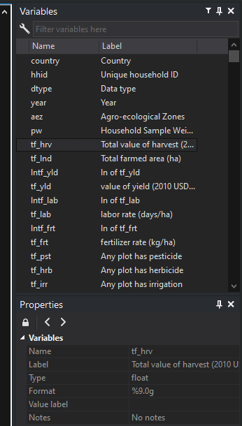
In the Stata command window, you can see the labels of variables in the Variables window as well as the Properties window. They also appear in the same place if you are looking at the data as a spreadsheet using Stata’s data editor.
Defining value labels
Variable labels describe the variable. Value labels describe what the numbers inside that variable mean.
Typical use cases:
- Binary indicators: 0 = no, 1 = yes
- Sex: 0 = male, 1 = female (or other encodings)
- Likert scales: 1 = strongly disagree … 5 = strongly agree
- Categories: 1 = urban, 2 = rural, etc.
There are two steps for value labels
- Define a value label (i.e., the mapping from numbers → text)
- Apply that value label to one or more variables
The syntax for defining a value label is a little tricky and I almost never remember it, so I have to use the drop down menu to get Stata to generate a little example and then I edit that example and place it in my code.
label define lblname # "label" [# "label" ...]
Here the syntax is:
label defineorlab deftells Stata you are defining a label for later uselblnameis the name of the value label set (you choose this)#is a numeric value (e.g., 0, 1, 2, 5)"label"is the text you want Stata to display for that numeric value
In our practice example, we would define a value label for use with the variable sex by writing:
* define label for sex
    lab def     sex_lbl 0 "Male" 1 "Female"
This creates a mappin 0 → "Male", 1 → "Female". It does not attach this mapping to any variable
Apply value label
Once you’ve defined a value label set, you need to attach it to the relevant variable(s). To apply a value label, the syntax is
label values varlist lblname
Here varlist is one or more variables and lblname is the label name that was defined when the labels were created.
Continuing with our example
* apply label to sex
    lab val     sex sex_lbl
Now if we were to descibe the sample data, we would see this:
variable name  storage  display  value
    name       type     format   label    variable label
----------------------------------------------------------------------
id             int       %9.0g             Individual ID
sex            byte      %8.0g   sex_lbl   =1 if respondent is female
wage           float     %9.0g             Hourly wage (USD)
You can also attach the value label to multiple variables at once, assuming each variable uses the same coding of what 0 and 1 represent:
* apply label to sex
    lab val     sex spouse sex_lbl
How value labels change what you see
The key point: value labels change what you see, not what is stored.
Stata still stores the underlying numeric values, but often displays the text labels instead.
In the Data Editor, suppose female is coded 0/1 and we’ve applied sex_lbl as above.
In the Data Editor, before applying the label, you would see something like:
| id | female |
|---|---|
| 1 | 1 |
| 2 | 0 |
| 3 | 1 |
| 4 | 1 |
After giving Stata lab val sex sex_lbl, the Data Editor would show
| id | female |
|---|---|
| 1 | Female |
| 2 | Male |
| 3 | Female |
| 4 | Female |
Stata will display the value labels, typically in blue text, but the underlying values are still stored as numerics (0 and 1). You just don’t see them by default.
If in the results window, you were to ask Stata to list id sex or tab sex (tab is the abbreviation for tabulate) the data, you would get:
     +--------------------+
     | id      sex        |
     |--------------------|
  1. |  1      Female     |
  2. |  2      Male       |
  3. |  3      Female     |
  4. |  4      Female     |
     +--------------------+
        sex |      Freq.     Percent        Cum.
------------+-----------------------------------
       Male |          1       25.00       25.00
     Female |          3       75.00      100.00
------------+-----------------------------------
      Total |          4      100.00
To see the underlying data values below the labels, you just add the option nolabel or nolab after the variable list. So list id sex, nolab produces:
     +--------------------+
     | id      female     |
     |--------------------|
  1. |  1          1      |
  2. |  2          0      |
  3. |  3          1      |
  4. |  4          1      |
     +--------------------+
And tab sex, nolab produces:
        sex |      Freq.     Percent        Cum.
------------+-----------------------------------
          0 |          1       25.00       25.00
          1 |          3       75.00      100.00
------------+-----------------------------------
      Total |          4      100.00
Common pitfalls and good habits
Pitfall 1: using strings instead of numeric with value labels
Bad pattern:
sexstored as string"Male"/"Female".
Better:
- Store as numeric:
female = 1if female,0if male
-
Attach a value label:
* define and assign value lables
  lab def       sex_lbl 0 "Male" 1 "Female"
  lab val       sex sex_lbl
Why numeric + value labels is better:
- arithmetic and statistics work correctly,
- sorting and filtering are more efficient,
- easier to merge and join datasets.
Pitfall 2: losing track of encodings
If you don’t label values, future-you must remember:
- Does
1mean “yes” or “no”? - Does
9mean “missing” or “other”?
Solution: label value sets that match the coding scheme:
* define and assign yes/no value labels
    lab def     yesno 0 "No" 1 "Yes"
    lab val     treated yesno
Pitfall 3: merging or appending two data sets with different value labels
Imagine you have data from Ethiopia and Nigeria that you want to combine into a single data set. Based on what you learned about tidy data, you have defined the largest political jurisdiction in both data sets as admin_1 because in Ethiopia they have regions and in Nigeria they have states. And based on what you learned about labeling, you’ve encoded admin_1 as a numeric (1, 2, 3, etc.). And to help you remember what these numbers mean, you’ve assigned a value label so that Stata displays the names of the regions/states instead of their identifying number.
However, if the first region in Ethiopia = 1 and the first state in Nigeria also = 1, you will get a problem when you merge or append these data. If you merge Nigeria into Ethiopia, the Ethiopia value label will be primary, meaning the Nigeria states suddenly get labelled with the Ethiopian names. Or if you merge Ethiopia into Nigeria, then the Nigeria value labels will override the Ethiopia labels.
Solution: If you think you might eventually combine different data sets, choose ID numbers that are unique to that data set. So, since Ethiopia comes before Nigeria in the alphabet, I can think of Ethiopia = 1 and Nigeria = 2. Then when I come to assigning identifiers to admin_1 in Ethiopia the first region takes the value 101 and in Nigeria the first state takes the value 201. This principle extends to identifying jurisdictions in admin_2, admin_3, etc.
In fact, this solution is a basic principle in generating unique IDs and it is why household or individual IDs in a data set are often so long. The IDs are frequently created by concatenating all the administrative jurisdictions together. For example, a household with ID 101040201 is likely the first household (household = 1) interviewed in the second level-3 administrative region (admin_3 = 2), which is the fourth level-2 administrative region (admin_2 = 4), which is in the first level-1 administrative region (admin_1 = 1), in the first country (country = 1). The zeros go into the ID because their are likely more than 9 adminitrative zones or households, meaning we need to use 01 instead of just 1 to get the IDs to have the same number of characters.
Summary
- Well-labeled data is vital for readability, sharing, and clear tables/graphs.
- Implement dataset, variable, and value labels systematically.
- Descriptive labels prevent confusion and errors months down the line.