Difference-in-Differences (DiD) is one of the most widely used methods for estimating causal effects in observational data. When we have panel data (repeated observations of the same units over time), DiD allows us to control for unobserved confounding factors that are constant over time (just like fixed effects).
This lecture covers:
- The intuition behind the 2x2 DiD model
- The critical “Parallel Trends” assumption
- Implementing DiD using Two-Way Fixed Effects (TWFE)
- Continuous Treatment DiD
We will use data from Cheng and Hoekstra (2013) on the “Castle Doctrine” laws (the expanded right to use lethal force in self-defense). The target is studying the effect of these laws (post = 1 after passing the law) on the natural log of the state’s homicide rate (l_homicide). Our panel identifier is state (sid) and our time metric is year.
The 2x2 DiD Model
The simplest DiD setup involves 2 groups (Treatment and Control) and 2 time periods (Pre-treatment and Post-treatment).
The intuition is that the Control group provides the counterfactual: it shows us what the trend in the outcome would have been for the Treatment group if they had not been treated.
A basic 2x2 DiD regression is: \(Y_{it} = \beta_0 + \beta_1 Treat_i + \beta_2 Post_t + \beta_3 (Treat_i \times Post_t) + \epsilon_{it}\)
- $\beta_1$ controls for baseline differences between the Treatment and Control groups.
- $\beta_2$ controls for the time trend common to both groups.
- $\beta_3$ is the Difference-in-Differences estimator—the causal effect of the treatment!
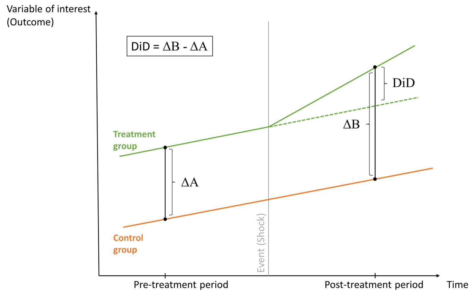
The graphic above highlights the core intuition of DiD. To isolate the causal effect of the intervention, we calculate three distinct differences:
- Pre-Difference ($\Delta A$): The baseline difference between the treatment and control groups prior to the intervention.
- Post-Difference ($\Delta B$): The difference between the actual outcomes of the two groups after the intervention.
- Difference-in-Differences (DiD Estimate): The difference between these two differences, yielding the effect of the intervention.
Visually, the DiD estimate is the gap between the actual outcome for the treated group and their counterfactual outcome (the dashed line, which assumes they followed the exact same trajectory as the control group in the absence of treatment).
* load the castle doctrine dataset
	use             "https://github.com/scunning1975/mixtape/raw/master/castle.dta", clear

* create time period dummy (1 for post-period)
	gen             after = (year >= 2006)

* create treatment group dummy (1 for states that ever passed a cdl law)
	gen             treat = (effyear != .)

* run the 2x2 did regression
	reg             l_homicide i.treat##i.after
While manually calculating the interaction with reg is great for understanding the mathematical mechanics, Stata 17+ has a dedicated suite of Difference-in-Differences commands. The didregress command automates the setup, calculates standard errors properly out-of-the-box, and naturally handles the uncollapsed, full panel dataset.
* use didregress on the uncollapsed panel
* syntax: didregress (depvar) (treatment_variable), group(group_id) time(time_id)
	didregress      (l_homicide) (post), group(sid) time(year) vce(hc2)
Parallel Trends Assumption
The validity of DiD hinges on the Parallel Trends Assumption: in the absence of treatment, the difference between the Treatment and Control groups would remain constant over time. We cannot test this directly (since we can’t observe the counterfactual), but we can look at pre-treatment periods to see if the groups were trending together before the intervention.
To visualize parallel trends, we compute the average outcome for both groups in each period and plot them.
* calculate means over time
	preserve
	collapse        (mean) l_homicide, by(treat year)

* parallel trends plot
	twoway      (connected l_homicide year if treat == 1, ///
                        lcolor(maroon)) ///
                    (connected l_homicide year if treat == 0, ///
                        lcolor(navy)), ///
                        xline(2005, lpattern(dash) ///
                        lcolor(black)) xtitle("Year") ///
                        legend(order(1 "Passed Castle Law" ///
                        2 "Never Passed"))  ///
                        ytitle("Log Homicide Rate") ///
                        title("Parallel Trends Check")
	restore
If the lines look roughly parallel before the treatment point (e.g., prior to 2005 when the first laws passed), the assumption is more plausible.
DiD with Two-Way Fixed Effects (TWFE)
When we have multiple time periods and staggered adoption (units getting treated at different times), the classic $2 \times 2$ formula doesn’t quite apply. Traditionally, economists handled this by estimating a Two-Way Fixed Effects (TWFE) regression. The post variable is equal to 1 if a state actively has the Castle Doctrine law that year, and 0 otherwise.
Here, $\alpha_i$ are unit fixed effects (replacing the $Treat$ dummy), $\gamma_t$ are time fixed effects and $D_{it}$ is the policy status dummy (post variable).
* set panel
	xtset           sid year

* twfe regression
	xtreg           l_homicide post i.year, fe vce(cluster sid)
The coefficient on post calculates the treatment effect holding both state and year averages constant.
The above is a very parsimonious specification. Now let’s replicate the full TWFE specification from Cheng and Hoekstra (2013) — the one that produces the headline finding of an ~8% increase in homicides will be our starting point for next lecture’s event study analysis.
First define global macros for the controls:
* define global macros
	global           crime1 jhcitizen_c jhpolice_c murder ///
                        homicide robbery assault burglary ///
                        larceny motor robbery_gun_r
	global           demo blackm_15_24 whitem_15_24 blackm_25_44 ///
                        whitem_25_44 //demographics
	global           lintrend trend_1-trend_51 //state linear trend
	global           region r20001-r20104  //region-quarter fe
	global           exocrime l_larceny ///
                        l_motor // exogenous crime rates
	global           spending l_exp_subsidy ///
                        l_exp_pubwelfare
	global           xvar l_police unemployrt poverty l_income ///
                        l_prisoner l_lagprisoner
	lab var			post "Year of treatment"
Now run the TWFE regression with the post variable and analytical weights. Analytical weights ([aweight=popwt]) tell Stata that each observation represents a different number of underlying units (here, state population). Larger states receive proportionally more weight — this is common in state-level panel studies where you want per-capita effects.
* set panel
	xtset           sid year

* full twfe specification
	xi: xtreg 		l_homicide post i.year $region $xvar ///
                        $lintrend [aweight=popwt], fe vce(cluster sid)
The coefficient on post is approximately 0.08, or an 8% increase in homicides. But this single coefficient tells us nothing about dynamics: Were homicides already rising before the law? Did the effect grow over time? In the next lecture, we will use event studies to answer these questions.
Continuous Treatment and Variations
Not all treatments are binary (0/1). You might have a continuous measure of treatment, such as the amount of gun sales in a state in a given year. In this case, continuous difference-in-differences applies:
* assuming a hypothetical continuous treatment variable 'gun_sales'
	xtreg           l_homicide c.gun_sales i.year $region $xvar ///
                        $lintrend [aweight=popwt], fe vce(cluster sid)
You can also interact your continuous treatment with a shock index (like passing a Castle Doctrine law) to isolate how the severity of a shock modulates the effectiveness of the treatment!
Summary
- Difference-in-Differences isolates the causal effect by subtracting a control group’s baseline trajectory from the treatment group.
- The Parallel Trends Assumption is critical: in the absence of treatment, both groups would have trended identically.
- Use ‘didregress’ or standard TWFE to calculate the specific deviation induced by the policy intervention.