Introduction to Stata & Github

Learning Objectives

Following this assignment students should be able to:

Fetch a branch, make commits, and push commits

Execute simple math in the Stata console

Import data in Stata

Assign and manipulate variables

Use built-in functions for math and stats

Visualize simple relationships between data

Reading

Topics

Using Github
The Stata interface
Importing data
Browsing and sorting data
Some basic commands
Asking for help

Readings

Reading: Github flow
Reading (just section 1.1): Getting started with Stata
Video (45 min): Ready. Set. Go Stata.

Lecture Notes

Exercises

Basic Expressions (10 pts)

Display the following calculations in the text editor.
1. 2 - 10
2. 3 * 5
3. 9 / 2
4. 5 - 3 * 2
5. (5 - 3) * 2
6. 4 ^ 2
7. 8 / 2 ^ 2
Run them by either clicking the Execute arrow button of the editor or press Ctrl+D (for do) (Windows) or Cmd+D (Mac) to run code and print the results in the console.

If no code is highlighted/selected this will run the entire file. If you highlighted/selected a block of code it will run that entire group of lines.

To tell someone reading the code what this section of the code is about, add a comment line that says ‘Exercise 1’ before the code that answers the exercise.
- Comments in Stata are added by adding the *#* sign. Anything after a * sign on the same line is ignored when the program is run.
- You can also create multiple lines of comments by starting the comment with /* and closing the comment with */.
- You can also create bookmarks using **# for the first level and **## for the second level.
So, the start of your program should look something like:
```
**# exercise 1

**## 1.1
display 2 - 10

**## 1.2
display 3 * 5
```
Basic Variables (5 pts)

Here is a small program that converts a price in U.S. dollars to a price in Euros and then prints out the resulting value.
```
    gen         p_usd = 2.62
    gen         p_euro = p_usd * 0.86
    display     p_euro
```
Create similar code to calculate the exchange rate between Euros and British Pounds.
- Start by creating an “empty” data set by typing set obs 1. This creates a single row in Stata’s data frame.
- Create a variable to store a price in Euros. Assign this variable a value of 5.87 (the price of a BigMac).
- Create a variable to store a price in Pounds. Assign this variable a value of 5.09.
- Calculate and print the exchange rate (the value of 1 Euro in GBP).
Data Basics (20 pts)

To get a sense of how to work with data and the types of data that Stata handles, we will look at a data set on life expectancy in 68 countries:

If the file lifeexp.dta is not already in your course folder then download it into your course folder.

Get familiar with the data by importing it using use then complete the following tasks. One thing to remember is that in Stata creating a variable requires one equal sign (=) while using logic expressions, like [if exp] requires two equal signs (==).
1. Describe the data (using describe). Which variable has a value label?
2. Calculate the mean life expectancy (using sum for summarize). What is the mean and standard deviation of life expectancy?
3. Calculate the median life expectancy (using the detail option to sum). What is median life expectancy?
4. Sort the data by country (using sort). Alphabetically, what is the first and last country in the data set?
5. List the regions in the data set (using tab for tabulate). How many regions are there?
6. Stata can label data (recall the region label). This means when you look at the data you see the label, but the label actually applies to a number. List the regions by their number (using the nolab option to tab). What number is assigned the label South America?
7. Calculate the mean life expectancy by region (using the prefix bys for bysort to the sum command). What is mean life expectancy in Europe and Central Asia?
8. Filter the data to calculate median population growth for North America (using the if [exp] conditional on sum). What is median population growth in the region?
9. Remove rows with null values of safewater (using drop if). How many observations were dropped?
10. Create a new data file called lifeexp_no-sw for no safewater (using save). What is the size in KB of this new file (look under data in the Properties Window)?
More Variables (5 pts)

Calculate GDP per capita for the US and then convert it to Euros. The GDP for the US is 30,490,000,000,000. The population of the US is 342,900,000. Use the echange rate from problem 2.
- Clear any data you might have loaded in Stata.
- Create an an new empty data set.
- Create a variable gdp and assign it the GDP of the US.
- Create a variable pop and assign it the population of the US.
- Create a variable gdp_pc and assign it a value by dividing GDP by population.
- Convert the value of gdp_pc into Euros and assign this value to a new variable.
- Display the final answer to the screen.
Built-in Functions (10 pts)

A built-in function is one that you don’t need to write yourself. Some come with the factory version of Stata while others are user written and must first be installed. Some examples include:
- abs() returns the absolute value of a number (e.g., abs(-2))
- round(), rounds a number (the first argument) to a given number of decimal places (the second argument) (e.g., round(12.1123, 0.01))
- sqrt(), takes the square root of a number (e.g., sqrt(4))
- strlower(), makes a string all lower case (e.g., strlower("HELLO"))
- strupper(), makes a string all upper case (e.g., strupper("hello"))
Use these built-in functions to display the following items:
1. The absolute value of -15.5.
2. 4.483847 rounded to one decimal place.
3. 3.8 rounded to the nearest integer. You don’t have to specify the number of decimal places in this case if you don’t want to, because round() will default to using 0 if the second argument is not provided.
4. "unemployment" in all capital letters.
5. "INFLATION" in all lower case letters.
6. The square root of 2.6 rounded to 2 decimal places by putting the sqrt() call inside the round() call.
Modify the Code (15 pts)

The following code explores wages and correlates using the National Longitudinal Surveys, Women sample, 1988. We will explore relationship in the entire data and then modify the code to explore differences in these relationships by union membership and college graduate.
```
    sysuse                  nlsw88.dta, clear
    sum                     wage hours
    tab                     married race, row
    bys married race:       sum wage hours           
```
Copy this code into your assignment and then add additional lines of code to calculate the following for union/non-union members and college grads/non-college grads:
1. Mean wage and hours (use bys and sum)
  1. For union members
  2. For non-union members
  3. For college grads
  4. For non-college grads
2. The percentage of Blacks who are (use tab)
  1. Union member
  2. Non-union members
  3. College grads
  4. Non-college gradss
3. Mean wage and hours of
  1. Union members who are college grads
  2. Union members who are non-college grads
  3. Non-union members who are college grads
  4. Non-union members who are non-college grads
Basic Graphs (15 pts)

Sticking with the National Longitudinal Surveys, Women sample, 1988, we are going to graph some of the relationships we just explored numerically.

1. Create a scatterplot in which hours is on the x-axis and wage is on the y-axis. Save the graph as a .png file (using graph export).

Stata’s default graphics scheme is pretty ugly. A number of users have developed their own, much more attractive, schemes. This also gives us a chance to load in user written packages. Stata maintains a repository of user written pacakges that can be installed within Stata from the internet. The one we are going to install is blindschemes. Then we will set that package’s graphic scheme as the default for our system.
```
ssc install blindschemes
set scheme plotplain, perm
```
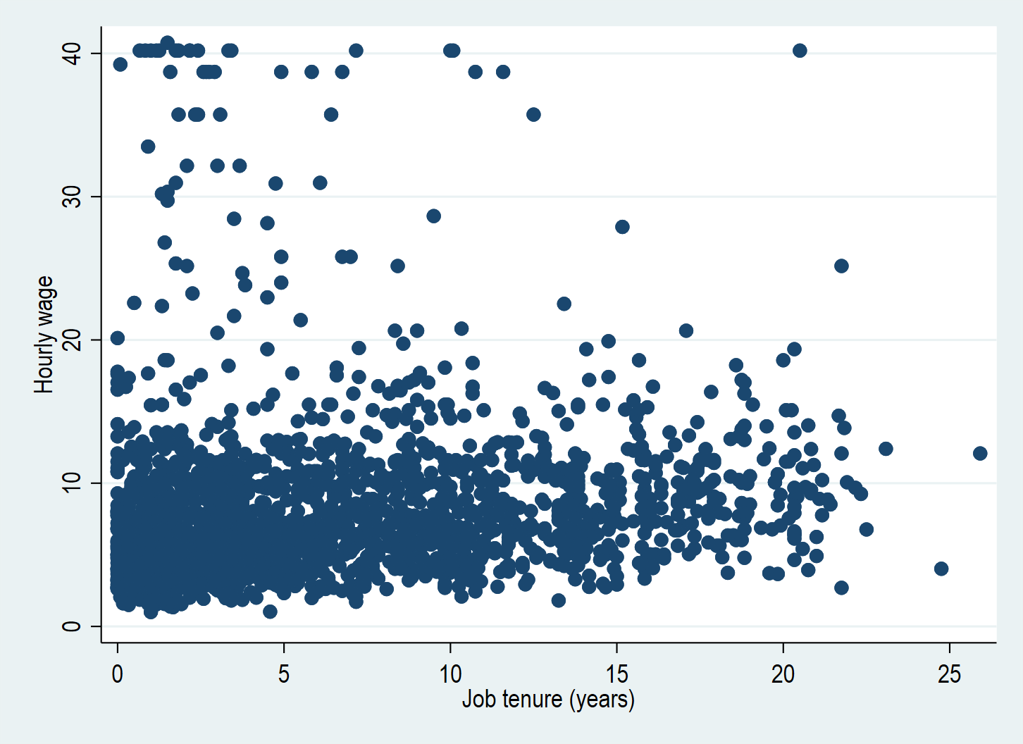
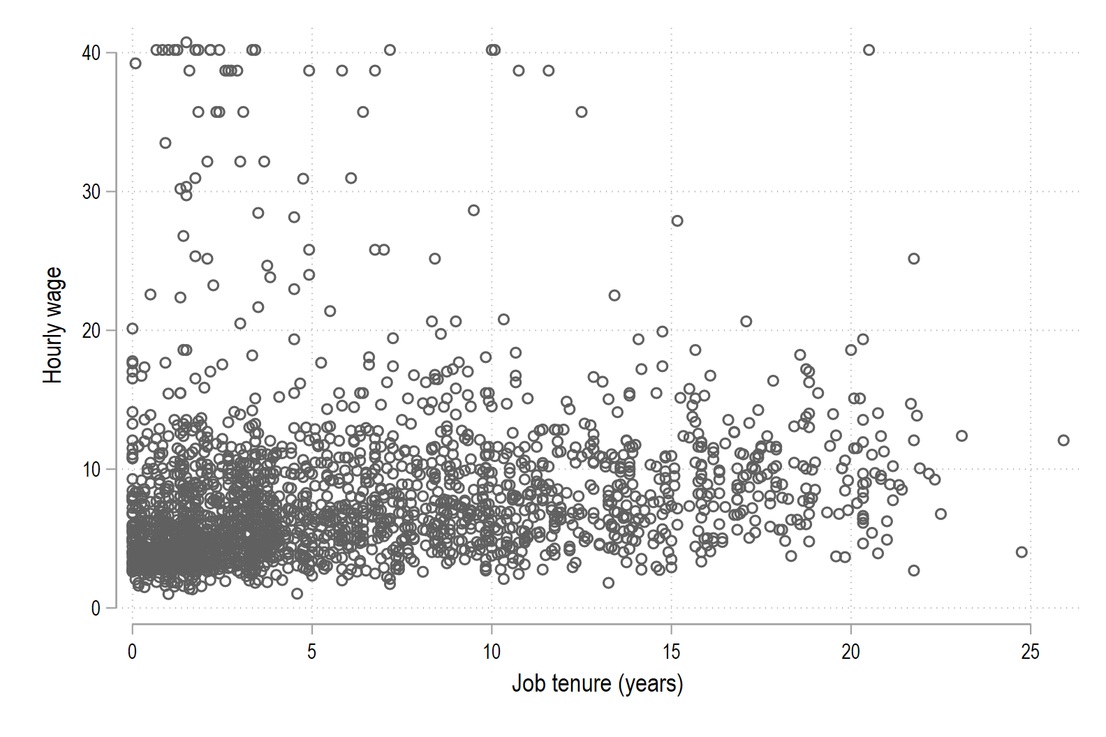
2. Create a scatterplot in which tenure is on the x-axis and wage is on the y-axis. Save the graph as a .png file.

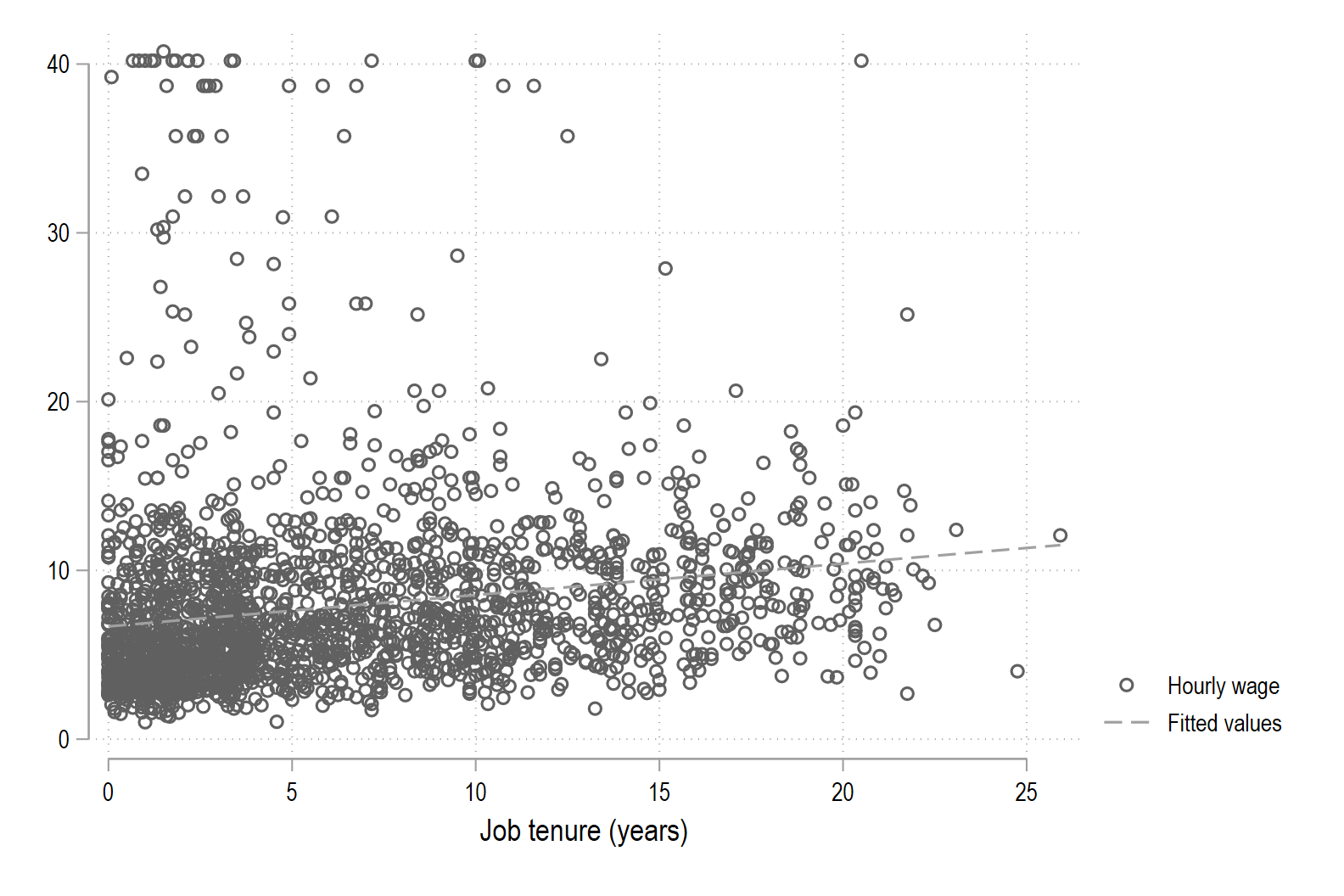
3. Add a line of best fit to the scatterplot using lfit. Use the command help twoway to open the help file. Scroll down to Definition and look for an example of putting two different types of graphs in the same region. Save the graph as a .png.
Check That Your Code Runs (20 pts)

Sometimes you think you’re code runs, but it only actually works because of something else you did previously. To make sure it actually runs you should save your work and then run it in a clean environment.

Follow these steps in to make sure your code really runs:
1. Restart Stata by closing the instance of Stata that you have open.
2. When you reopen Stata, type in the command line clear all. Or, better yet, put clear all at the top of your .do file, after the preamble but before any commands.
3. Rerun your entire homework assignment by clicking the Execute button to make sure it runs from start to finish and produces the expected results.
4. Make sure that you saved your code with the name of the assignment number (i.e., assignment_01). You should see the file in your git repo on your machine.
5. Make sure that your code will run on other computers (relevant for all assignments after the first assignment)
  - No cd. Use a project.do file instead to set directories
  - Use only relative paths in files other than the project.do file
  - Use / not \ for paths
Challenge 1 (Challenge - 10 pts)

Sticking with the National Longitudinal Surveys, Women sample, 1988, we are going to graph some of the relationships we just explored numerically.

Using only code that you write in .do files and the help twoway command, create the following graphs:
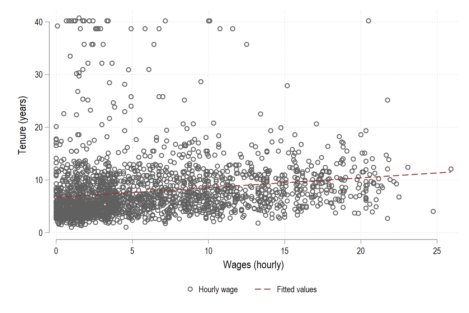
1. Create a scatterplot in which tenure is on the x-axis and wage is on the y-axis. Add a line of best fit to the scatterplot using lfit. Change the color of that line to maroon. Label the x-axis as Tenure (years) and the y-axis as Wages (hourly). Then create a legend that is two columns and place the legend below the graph (in the 6 o’clock position). Save the graph as a .png.

Assignment submission checklist

Assignment

Learning Objectives

Reading

Topics

Readings

Lecture Notes

Exercises

Solutions