Learning Objectives
Following this assignment students should be able to:
- Understand data structure
- Label variables
- Create and assign label values to data
- Create new variables
- Manipulate existing variables
- Append and marge two data sets together
Reading
Topics
- Types of data
- Labeling data
- Creating and manipulating data
- Joining data
Readings
- Reading (chapter 5): Research Ethics for Applied Economics
- Reading: Data Management
- Video (5 min): How to merge files into a single dataset
Lecture Notes
Exercises
-
Messy Data (10 pts)
A lot of real data isn’t very tidy, mostly because most scientists aren’t taught about how to structure their data in a way that is easy to analyze.
Download an untidy version of the World Bank data on GDP, which includes countries, years, and meta data.
Think about what could be improved about this data and write down answers to the following questions:
- Describe three things about this data that are not tidy and how you could fix each of those issues.
- Could this data easily be imported into a programming language or a database in its current form?
- Do you think it’s a good idea to enter the data like this and clean it up later, or to have a good data structure for analysis by the time data is being entered? Why?
-
Clean Up (10 pts)
Convert the World Bank data downloaded in Exercise 1 into a more tidy format.
-
Label Variables (10 pts)
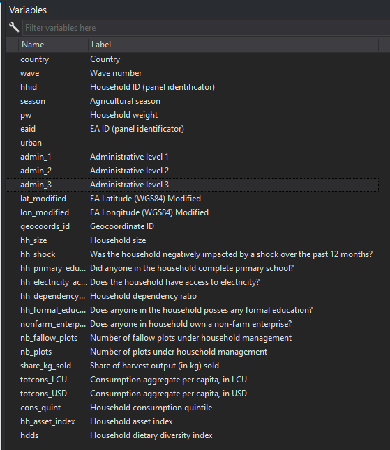
Download the World Bank’s Living Standards Measurement Survey (LSMS) household data set. The data includes the following variables (among others):
- Identifiers & structure
country– country codewave– survey wave (e.g., 1, 2)hhid– household IDeaid– enumeration area ID (cluster)season– season of interview (e.g., lean, harvest)
- Location
urban– urban (=1) or rural (=0)admin_1,admin_2,admin_3– administrative unitslat_modified,lon_modified– household GPS coordinatesgeocoords_id– identifier for GPS cluster
- Household characteristics
hh_size– household size (number of members)hh_shock– indicator that hh experienced a shockhh_primary_education– indicator: head has at least primary schoolinghh_electricity_access– indicator: hh has electricityhh_dependency_ratio– dependents / working-age membershh_formal_education– years of formal education of the headnonfarm_enterprise– indicator: household runs a nonfarm enterprisenb_fallow_plots– number of fallow plotsnb_plots– number of cultivated plotsshare_kg_sold– share of agricultural production sold
- Welfare
totcons_LCU– total consumption (local currency)totcons_USD– total consumption (USD)cons_quint– consumption quintile (1 = poorest, 5 = richest)hh_asset_index– asset indexhdds– household dietary diversity score
Apply the following labels to the corresponding variable
- Country ->
country - Wave number ->
wave - Agricultural season ->
season - Administrative level 1 ->
admin_1 - Administrative level 2 ->
admin_2 - Administrative level 3 ->
admin_3 - Household size ->
hh_size - Was the household negatively impacted by a shock over the past 12 months? ->
hh_shock - Did anyone in the household complete primary school? ->
hh_primary_education - Does the household have access to electricity? ->
hh_electricity_access - Household dependency ratio ->
hh_dependency_ratio - Does anyone in the household posses any formal education? ->
hh_formal_education - Does anyone in household own a non-farm enterprise? ->
nonfarm_enterprise - Number of fallow plots under household management ->
nb_fallow_plots - Number of cultivated plots under household management ->
nb_plots - Share of harvest output (in kg) sold ->
share_kg_sold - Consumption aggregate per capita, in LCU ->
totcons_LCU - Consumption aggregate per capita, in USD ->
totcons_USD - Household consumption quintile ->
cons_quint - Household asset index ->
hh_asset_index - Household dietary diversity index ->
hdds
- Identifiers & structure
-
Label Values (10 pts)
Using the World Bank’s LSMS data,
1. Define a value label set called
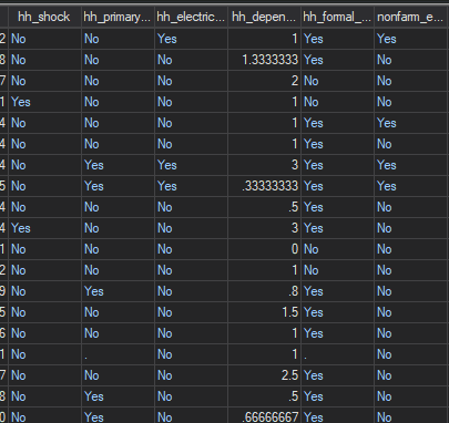
yesnowhere0 = Noand1 = Yes2. Assign the value label set
yesnoto the following variables:hh_shockhh_primary_educationhh_electricity_accesshh_formal_educationnonfarm_enterprise
Defining value labels when there are just a couple options (yes/no, male/female) is fairly straightforward, especially when variables are already binary (0/1). But sometimes a variable already exists that has the information we want, just not in the form we want. In that case, we can create a new, intermediate variable, whose values are based on the existing variable. This allows us to change one form of data (strings) into another form (numeric) and then apply labels.
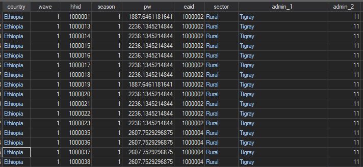
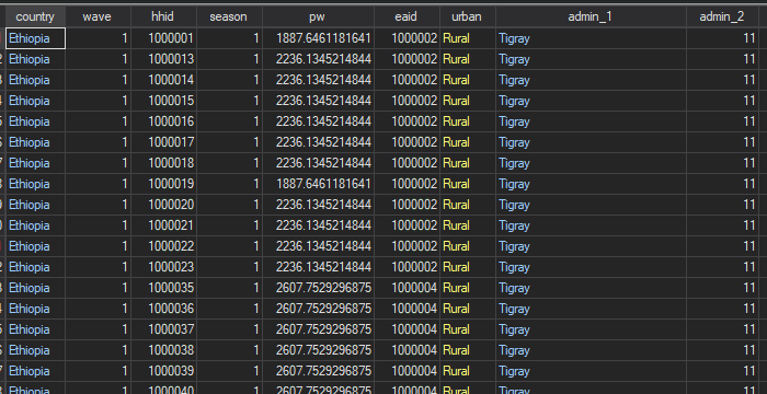
3. Create a variable called
sectorthat equals 0 ifurban = Ruraland equals 1 ifurban = Urban.- Label that variable “EA is rural or urban”
- Define a value label set called
sec_lblwhere0 = Ruraland1 = Urban - Assign the value label set
sec_lblto the variablesector - Drop
urbanand placesectoraftereaid(usehelp orderif you need help with theordercommand)
Defining value labels in this way when there are a lot of options can become very tedious very quickly. Luckily, Stata has a decode/encode command that can sometimes creatly reduce the amount of coding you have to do to define and assign a label.
You will often have a variable which is a string that you would like to convert to a numeric. As an example, you can think of a variable called
statethat takes values of the name of each state in the U.S. In order to use this information in a regression, we need to convert the string to a numeric, like we did withsector. But with 50 state names, it will take a long time to 1) create a new variable that takes a unique numerical value for each state name and 2) define a label set for every value.In this case, we can use
encodeto change the strings to numerical values and then use the string text as a value label for each numerical value. The syntax for the command is:encode varname, gen(newvar)where
varnameis the name of the existing string variable andnewvaris the new, numerical variable you want to create.4. Encode the variable
countryso that it is a numerical variable and uses the string values as labels.- Call the new variable you create
Country - Drop the old variable
country - Rename
Countryascountry - Use the command
orderto placecountryas the first variable in the data set
5. Encode the variable
admin_1so that it is a numerical variable and uses the string values as labels. Follow the same steps as in 4.4 and useorderto place the newadmin_1immediately in front ofadmin_2.
-
Create Variables (10 pts)
Using the World Bank’s LSMS data,
1. Create a new variable called
tot_plotsthat combines cultivated and fallow plots usingegen. Label the new variable with “Total number of plots under household management”. What is the mean number of plots owned by a household?2. Compute the mean total consumption in dollars (
meancons_USD) for each consumption quintile using theby()option along withegen. Label the new variable with “Mean consumption per quntile (USD)”. Usingtab, what is the mean consumption for the highest and lowest quintile?3. Find the maximum household dietary diversity score (
hdds) separately for households with and without electricity access. Call this new variablemax_hddsand label it “Max HDDS by electricity access”. (To get this, usesumand and thebysortprefix, which can be abbreviatedbys. So, the line of code would startbys hh_electricity_access: sum).
-
Change Variables (10 pts)
Before undertaking this exercise, make sure you save the household-level version of that data that is currently in Stata’s memory. Save the file into your data folder and call it
household_all.dta. Make sure you use the optionreplaceso that when you run the.dofile again it writes over any pre-existing versions of the data.Using the World Bank’s LSMS data, use
collapseto create an EA-level dataset (grouped byeaidandsector) that contains the following EA-level variables:- Mean household size: based on
hh_size - Share of households with electricity: based on
hh_electricity_access - Share of households with a nonfarm enterprise: based on
nonfarm_enterprise - Mean total consumption in USD: based on
totcons_USD
After the collapse, rename these variables as
ea_hh_sizeea_electricity_accessea_nonfarm_enterpriseea_totcons_USD
-
What is the average EA-level household size in urban and rural areas?
-
What percentage of urban households, on average, have electricity access? What percentage of rural households, on average, have electricity access?
-
What percentage of urban households, on average, have a non-farm enterprise? What percentage of rural households, on average, have a non-farm enterprise?
-
Is average EA-level consumption (
mean_totcons_usd) higher in urban or rural areas?
Save this EA-level file as
ea_summary.dta.
- Mean household size: based on
-
Append Data (10 pts)
Using the World Bank’s LSMS data, we are going to simulate the common case where survey data arrive as separate files by wave. In fact, this is how the LSMS data comes, I’ve just given you a data set in which all the waves and all the countries have already been appended into a single data set. You will create wave-specific datasets and then append them.
Start by re-loading the household data (
household_all.dta). Create a data set that contains only observations from wave 1 using thekeep ifcommand. Save this file ashh_wave1.dta.1. How many observations came from the waves that are NOT wave 1?
Now, re-open the full dataset and keep only wave 2 observations and save this as
hh_wave2.dta.2. How many observations came from the waves that are NOT wave 2?
Finally, append the data set that contains just wave 1 to the data set that contains just wave 2 using
append.3. How many observations are in the combined wave 1 and wave 2 data set?
-
Merge Data (20 pts)
Using the World Bank’s LSMS data, we are going to practice merging datasets that represent different levels of aggregation (EA-level and household-level). Start by loading the
ea_summary.dtafile that you created in exercise 6. This will be the master file in memory.1. Use
isidto determine what variable(s) uniquely identify the data. What are these variable(s)?Think through the structure of the EA and household data:
- In the EA summary dataset, each
eaid–sectorcombination should appear once. - In the household dataset, each
eaidappears many times (one row per household).
This suggests a one-to-many merge: many households per EA, one EA-level summary per EA. Now merge the household data into the EA data.
2. How many matched and unmatched observations are there?
Now each household observation contains both:
- Household-level variables (e.g.,
totcons_USD,hh_dependency_ratio), and - EA-level averages (
mean_totcons_usd,mean_dep_ratio, etc.).
3. Create a consumption gap variable called
cons_gapthat is total household consumption (USD) minus mean consumption at the EA. This measures how much a household’s consumption differs from the average consumption in its EA. Is the consumption gap larger for rural households or urban households?**Save this merged data set as
household_ea.dta.
- In the EA summary dataset, each
-
Check That Your Code Runs (10 pts)
Sometimes you think you’re code runs, but it only actually works because of something else you did previously. To make sure it actually runs you should save your work and then run it in a clean environment.
Follow these steps in to make sure your code really runs:
-
Restart Stata by closing the instance of Stata that you have open.
-
When you reopen Stata, type in the command line
clear all. Or, better yet, putclear allat the top of your.dofile, after the preamble but before any commands. -
Rerun your entire homework assignment by clicking the
Executebutton to make sure it runs from start to finish and produces the expected results. -
Make sure that you saved your code with the name of the assignment number (i.e.,
assignment_01). You should see the file in your git repo on your machine. -
Make sure that your code will run on other computers (relevant for all assignments after the first assignment)
- No
cd. Use aproject.dofile instead to set directories - Use only relative paths in files other than the
project.dofile - Use
/not\for paths
- No
-
-
Challenge 3 (Challenge - 20 pts)
Using the
household_ea.dtadata set that you created in exercise 8, we are going to dig a bit more into the consumption gap between households in rural and urban EAs. We will walk through a number of steps that require you to use the concepts and commands from earlier in Assignment 3.- Start by using
gento create a variable calledgapthat equals 1 if the household’s consumption gap is negative. Thenreplacethe value ofgapso that it equals 0 if the household’s consumption gap is positive.- Hint: there are a number of households with missing values because either the household or EA data was missing. For reasons that are not important, Stata treates a missing value (the sysmis
.) as positive infinity. So if you were to just typereplace gen = 0 if cons_gap > 0Stata will assign a 0 to household above the mean consumption but also to all households with missing values. So you need to add an additional conditional aboutcons_gapnot equalling.
- Hint: there are a number of households with missing values because either the household or EA data was missing. For reasons that are not important, Stata treates a missing value (the sysmis
- Label the variable as
Indicator for sign of consumption gap. Also define a value label calledgap_lblwhere 0 isPositive Gapand 1 isNegative Gap. Assign this value label to thegapvariable. - Use
egento create a variable calledbelowthat totals up all households withgap = 1. Do this byeaidandsector. Label the variableNumber of households below mean consumption. - Use
egento create a variable calledabovethat totals up all households withgap = 0. Do this byeaidandsector. Label the variableNumber of households above mean consumption.- Hint: when having Stata total up households with a positive gap, you need to explicitly tell Stata to count the households where
gap == 0.
- Hint: when having Stata total up households with a positive gap, you need to explicitly tell Stata to count the households where
- Use
egento create a variable calledtot_hhthat counts up all households in an EA and sector. Label the variableTotal number of households in EA. - Use
gento create a variable calledshare_belowthat is the percentage of households with a negative consumption gap within an EA and sector. Label the variablePercentage of households in EA below mean consumption.
Now that we have all these variables created and labeled, we can ask questions about where the gap is most negative or most positive using
bysin combination withsum.- Is the share of households with a negative consumption gap greater in urban or rural EAs?
- Which country has the largest share of households with a negative consumption gap?
- Which country has the smallest share of households with a negative consumption gap?
- Start by using
Assignment submission checklist
Solutions
- Messy Data
- Clean Up
- Label Variables
- Label Values 1, 2, 3
- Create Variables
- Change Variables
- Append Data
- Merge Data
- Check That Your Code Runs
- Challenge 3